Beneath the bottom of the Bogoliubov sea

Because of the quasiparticle-quasihole symmetry (Sec. 3), the spectrum of the HFB Hamiltonian contains as many negative as positive eigenvalues. Therefore, the HFB equation (7) constitutes an eigenvalue problem for the operator unbounded from below, and the HFB spectrum extends from minus to plus infinity, see Fig. 1. Moreover, one-body densities (density matrix and pairing tensor) are given by infinite sums over all negative-energy (quasihole) states, cf. Eq. (9). In analogy to the Fermi sea of occupied states, which appears in the Hartree-Fock (HF) theory, we call the set of quasihole states the Bogoliubov sea. Note again that the Fermi sea extends over a finite range of energies - from the bottom of the HF potential up to the Fermi energy - whereas the Bogoliubov sea is infinitely deep, in a nice analogy with the sea of one-electron states of the relativistic Dirac equation.

In practice, since infinite sums over the Bogoliubov sea cannot be carried out, the number of pairing-active states must be truncated. Two different ways of achieving this goal are most often implemented, namely, solution of the HFB equations in a finite s.p. space (e.g., the so-called two-basis method[22]) and truncation of the summation in the quasiparticle space. The second method correspond to creating an artificial finite bottom of the Bogoliubov see. In this section we discuss the consequences of neglecting the quasihole states that are below the bottom of that sea[23,24].

The main problem concerns the calculation of the pairing tensor, which is the sum of products of upper and lower components of quasihole states, cf. Eq. (9). When this sum is performed over the infinite complete set of quasiparticle states, the resulting pairing tensor is antisymmetric, while for truncated sums it may acquire a symmetric part. Usually the symmetric component is small;[23] hence, can be neglected. However, its very existence means that the many-fermion state which would have had such a pairing tensor simply does not exist. The smallness of the symmetric part can be deceiving, because the symmetric pairing tensor corresponds to a many-boson system. Consequently, appearance of the symmetric component implies the violation of the Pauli principle. This is a potentially dangerous situation - within a variational theory one should avoid the boson sector whose ground state is way below the fermionic ground state.

A solution to this problem[23], discussed below, consists in marrying the two truncation methods mentioned above. That is, we shall first use the quasiparticle truncation method to define the appropriate s.p. cutoff, and then the HFB equations are solved in this truncated space, leading to a perfectly antisymmetric pairing tensor.

Let us consider the case of truncated summations over the Bogoliubov sea and assume that we have kept only $K$ quasihole states. In order to maintain the quasiparticle-quasihole symmetry, we apply the same truncation to quasiparticle and quasihole states, that is, we also keep $K$ quasiparticle partner states. This is convenient, and always possible, because the quasiparticle (unoccupied) states do not impact HFB densities. Then, matrix ${\cal{}U}$ becomes rectangular - it has less columns ($2K$) than rows. Since all kept quasiparticle and quasihole states are orthonormal, we still have ${\cal{}U}^+{\cal{}U} = 1$. However, since now the quasiparticle space is not complete, ${\cal{}U}$ is not anymore unitary, and the product ${\cal{}U}{\cal{}U}^+ = {\cal{}P}$ is not equal to unity. All what remains is the hermitian and projective property of ${\cal{}P}$:

$${\cal{}P}^+={\cal{}P}, \quad {\cal{}P}^2={\cal{}P}.$$ (10)

Since $\mbox{Tr}{\cal{}P}=2K$, ${\cal{}P}$ has exactly $2K$ eigenvalues equal to 1.

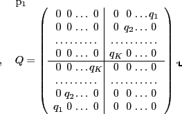
In its explicit form, matrix ${\cal{}P}$ reads:

$${\cal{}P} = \left(\begin{array}{cc} P & Q \\ Q^* & P^* \e... ...V^*U^T \\ VU^+ + U^*V^T, & VV^+ + U^*U^T \end{array}\right).$$ (11)

In terms of $P$ and $Q$, Eqs. (10) can be written as:

$$P^+ = P, \quad Q^T = Q \quad\mbox{and}\quad P^2 + QQ^+ = P, \quad PQ + QP^* = Q,$$ (12)

where $\mbox{Tr}{P}=K$.

Properties of matrices $P$ and $Q$ can be most easily discussed in the particle basis that diagonalizes $P$. Suppose that column $f$ is an eigenvector of $P$ with eigenvalue $p$, that is, $Pf = pf$. From Eqs. (12) it follows that $p$ must be between 0 and 1. Moreover, if $Qf^*$ is not equal to zero, then $Qf^*$ is an eigenvector of $P$ with eigenvalue 1$-$$p$, that is, P $(Qf^*) = (1-p)Qf^*$. Conversely, if $Qf^*$ is equal to zero, than $p$=0 or $p$=1.

Altogether, the spectrum of $P$ can be divided into three regions: (i) $i$ states with $p_\nu$=1, where all matrix elements of $Q$ vanish, $Q_{\nu\nu'}$=0, (ii) $2k$ states with 0$<$$p_\nu$$<$1, where eigenvectors are arranged in pairs $p_{\tilde{\nu}}$=1$-$$p_{\nu}$ such that the only non-vanishing matrix elements of $Q$ are

$$Q_{\nu\tilde{\nu}} = Q_{\tilde{\nu}\nu} = q_{\nu} = \sqrt{p_{\nu}(1-p_{\nu})},$$ (13)

and (iii) states with $p_\nu$=0, where again all matrix elements of $Q$ vanish. In practical calculations of solving the HFB equation in infinite-dimensional quasiparticle spaces (like the coordinate representation), the first region almost never appears ($i=0$), and then $k=K$. However, for truncated quasiparticle spaces, the third region always exists and contains the null space of $P$.

We now see that when $K$ quasiparticles are included in the quasiparticle space and $i=0$, in the particle space there appears a basis of 2$K$ s.p. states, which we call natural basis. Each state in the first half of the natural basis has its partner in the second half. By ordering the eigenvalues of $P$ and neglecting the zero eigenvalues for $\nu>2K$, we can write matrices $P$ and $Q$ in a general form:

$$P=\left( \begin{array}{c@{\hspace{\di}}c@{\hspace{\di}}c@{\h... ... & 0 & \ldots & 0 & 0 & 0 & \ldots & 0 \\ \end{array}\right).$$ (14)

If there appear $i>0$ states with $p_\nu=1$, the number of paired states decreases to $2k=2K-2i$ and the size of the natural basis decreases to $i+2k=2K-i$.

The HFB equations can now be solved in the finite natural basis, whereupon the pairing tensor becomes exactly antisymmetric and the dangerous violations of the Pauli principle are removed exactly[23]. The advantage of this method is in the fact that the truncated s.p. space is not arbitrarily cut but it is adjusted to the truncated quasiparticle space.