Applications

When compared to the experimental binding energies, the quasilocal Skyrme functional HFB-17 [18] (Fig. 6) gives results, which have the quality very similar to those given by the nonlocal Gogny functional D1M [19] (Fig. 7). In both cases, the functionals were augmented by terms responsible for the pairing correlations and all parameters were adjusted specifically to binding energies. Moreover, in both cases, by using either the 5D collective Hamiltonian approach or configuration mixing, theoretical binding energies were corrected for collective quadrupole correlations. The results are truly impressive, with the RMS deviations calculated for 2149 masses being as small as 798 and 581keV, respectively.

Figure 6: Differences between measured [20] and HFB-17 [18] masses, as a function of the neutron number $N$. Reprinted figure with permission from Ref. [18]. Copyright 2009 by the American Physical Society.

Figure 7: Differences between measured [20] and D1M [19] masses, as a function of the neutron number $N$. Reprinted figure with permission from Ref. [19]. Copyright 2009 by the American Physical Society.

The problem of treating collective correlations and excitations within the DFT or EDF approaches is one of the most important issues currently studied in applications to nuclear systems. The question of whether one can describe these effects by using the functional only is not yet resolved. In practice, relatively simple functionals that are currently in use, require adding low-energy correlation effects explicitly. This can be done by reverting from the description in terms of one-body densities back to the wave functions of mean-field states. For example, for quadrupole correlations this amounts to using the following configuration-mixing states,

$$\vert\Psi_{NZ,JM}\rangle = \int {\rm d}\beta{\rm d}\gamma \s... ...P}_N \hat{P}_Z \hat{P}_{JMK} \vert\Psi(\beta,\gamma) \rangle ,$$ (9)

where $\hat{P}_N$, $\hat{P}_Z$, and $\hat{P}_{JMK}$ are projection operators on good neutron number $N$, proton number $Z$, and angular momentum $J$ with laboratory and intrinsic projections $M$ and $K$. The intrinsic mean-field wave functions $\vert\Psi(\beta,\gamma) \rangle$ correspond to one-body densities constrained to quadrupole deformations $\beta$ and $\gamma$ [21].

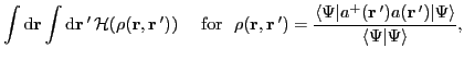
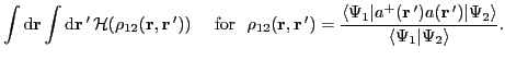
To determine variationally the mixing amplitudes $f_K(\beta,\gamma)$, one has to generalize the energy densities, such as those shown in Eqs. (4)-(7), to transition energy densities that enable us to compute Hamiltonian kernels. For mean-field states, this can be rigorously done by using the Wick theorem, whereby the average energy $\langle\Psi\vert\hat{H}\vert\Psi\rangle$ generalizes to matrix element $\langle\Psi_1\vert\hat{H}\vert\Psi_2\rangle$ as [21]:

$$\langle\Psi\vert\hat{H}\vert\Psi\rangle \simeq \int{\rm d}\vec{r}\int{\rm d}\vec{r}\,'\,{\cal H}(\rho(\vec{r},\v... ...^+(\vec{r}\,')a(\vec{r}\,')\vert\Psi\rangle} {\langle\Psi \vert\Psi\rangle}} ,$$ (10)

$$\langle\Psi_1\vert\hat{H}\vert\Psi_2\rangle \simeq \int{\rm d}\vec{r}\int{\rm d}\vec{r}\,'\,{\cal H}(\rho_{12}(\vec{... ...c{r}\,')a(\vec{r}\,')\vert\Psi_2\rangle} {\langle\Psi_1 \vert\Psi_2\rangle}} .$$ (11)

Although for densities of correlated states, which are employed in DFT or EDF methods, this prescription cannot be properly justified, it has been successfully used in many practical applications. However, even this simple prescription creates problems [22], which may require implementing more complicated schemes [23].

Figure 8: Scatter plot comparing the theoretical and experimental $2^+_1$ excitation energies of the 359 nuclei included in the survey of Ref. [24]; picture courtesy of M. Bender.

Figure 9: Theoretical $2^+_1$ excitation energies of 537 even-even nuclei as a function of their experimental values [25]. Reprinted figure with permission from Ref. [13]. Copyright 2010 by the American Physical Society.

An example of the results is shown in Fig. 8, where calculated $2^+_1$ excitation energies [24] are compared with experimental data. One obtains fairly good description for nuclei across the nuclear chart. Calculations slightly overestimate the data, which is most probably related to the fact that in this study the nonrotating mean-field states were used, see Ref. [26] and references cited therein. As shown in Fig. 9, this deficiency disappears when the moments of inertia of the 5D collective Hamiltonian are determined by using infinitesimal rotational frequencies [13]. At present, calculations using in light nuclei the triaxial projected states of Eq. (9) are becoming possible for the relativistic (Fig. 10) and quasilocal (Fig. 11) functionals.

Figure 10: Energies and the average axial deformations for the lowest quadrupole states in $^{24}$Mg, together with the mean-field (dotted) and the angular-momentum-projected energy curves and squares of collective wave functions. Reprinted figure with permission from Ref. [27]. Copyright 2010 by the American Physical Society.

Figure 11: Excitation spectra and B(E2) values in e$^2$fm$^4$ compared to the available experimental data in $^{24}$Mg. The spectrum is subdivided into a ground-state band, a $\gamma$ band, and additional low-lying states that do not necessarily form a band. From Ref. [28]; picture courtesy of M. Bender.

Another fascinating collective phenomenon that can presently be described for the non-local [29,30] and quasilocal functionals [31] is the fission of very heavy nuclei. In Fig. 12, an example of fission-path calculations performed in $^{258}$Fm is shown in function of the elongation and shape-asymmetry parameters. One obtains correct description of the region of nuclei where the phenomenon of bimodal fission occurs and predicts regions of the trimodal fission, see Fig. 13.

Figure 12: The energy surface of $^{258}$Fm calculated for the quasilocal EDF as a function of two collective variables: the total quadrupole moment $Q_{20}$ representing the elongation of nuclear shape, and the total octupole moment $Q_{30}$ representing the left-right shape asymmetry. Indicated are the two static fission valleys: asymmetric path aEF and symmetric-compact path sCF. From Ref. [32]; picture courtesy of A. Staszczak.

Figure 13: Summary of fission pathway results obtained in Ref. [31]. Nuclei around $^{252}$Cf are predicted to fission along the asymmetric path and those around $^{262}$No along the symmetric path. These two regions are separated by the bimodal symmetric fission around $^{258}$Fm. In a number of the Rf, Sg, and Hs nuclei, all three fission modes are likely (trimodal fission). From Ref. [31]

In recent years, significant progress was achieved in determining the multipole giant resonances in deformed nuclei by using the RPA and QRPA methods. In light nuclei, the multipole modes can be determined for the nonlocal, relativistic, and quasilocal functionals, see Figs. 14, 15, and 16, respectively. In heavy nuclei, such calculations are very difficult, because the number of two-quasiparticle configurations that must be taken into account grows very fast with the size of the single-particle phase space. Nevertheless, the first calculation of this kind has already been reported for $^{172}$Yb, see Fig. 17. The future developments here will certainly rely on the newly developed iterative methods of solving the RPA and QRPA equations [33,34,35].

Figure 14: Dipole excitations in $^{24}$Mg determined for the nonlocal Gogny D1S functional. From Ref. [36]; picture courtesy of S. Péru.

Figure 15: Dipole excitations in $^{20}$Ne determined for the relativistic NL3 functional. Reprinted figure with permission from Ref. [37]. Copyright 2008 by the American Physical Society.

Figure 16: Quadrupole excitations in $^{24}$Mg determined for the quasilocal Skyrme SkM* functional. Reprinted figure with permission from Ref. [38]. Copyright 2008 by the American Physical Society.

Figure 17: Dipole excitations in $^{172}$Yb determined for the quasilocal Skyrme SkM* functional. From Ref. [39]; picture courtesy of J. Terasaki.

The EDF methods were also recently applied within the full 3D dynamics based on the time-dependent mean-field approach. In Ref. [40], the spin-independent transition density was calculated in the 3D coordinate space for the time-dependent dipole oscillations. It turned out that one of the Steinwedel-Jensen's assumptions [41], $\delta\rho_n(\vec{r};t)=-\delta\rho_p(\vec{r};t)$, was approximately satisfied for $^8$Be. In contrast, in $^{14}$Be, large deviation from this property was noticed. Figure 18 shows how transition densities $\delta\rho_n(\vec{r};t)$ (lower panels) and $\delta\rho_p(\vec{r};t)$ (upper panels) evolve in time in the $x$-$z$ plane. The time difference from one panel to the next (from left to right) roughly corresponds to the half oscillation period. White (black) regions indicate those of positive (negative) transition densities. One sees that significant portions of neutrons actually move in phase with protons.

An interesting 3D EDF time-dependent calculation was recently performed for the $\alpha$-$^8$Be fusion reaction [42]. Although this calculation aimed at elucidating properties of the triple-$\alpha$ reaction, it was performed at the energy above the barrier, where the time-dependent mean-field approach can lead to fusion, whereas the real triple-$\alpha$ reaction involves tunneling through the Coulomb barrier. Nevertheless, the studied tip-on initial configuration in the entrance channel, shown in the upper panel of Fig. 19, is probably the preferred one as it must correspond to the lowest barrier. The calculations lead to the formation of a metastable linear chain state of three $\alpha$-like clusters which subsequently made a transition to a lower-energy triangular $\alpha$-like configuration before acquiring a more compact final shape, as shown in the lower panels of Fig. 19.

Figure 18: Nuclear TDHF transition densities in $^{14}$Be, see text. Reprinted from Ref. [40], Copyright 2007, with permission from Elsevier.

Figure 19: Nuclear TDHF densities in $^{12}$Be, see text. Reprinted figure with permission from Ref. [42]. Copyright 2010 by the American Physical Society.