Next: Bibliography
P. Baczyk, J. Dobaczewski, M. Konieczka, W. Satula, T. Nakatsukasa, and K. Sato
Date: February 3, 2017
Similarity between the neutron-neutron (![]() ), proton-proton (
), proton-proton (![]() ), and
proton-neutron (
), and
proton-neutron (![]() ) nuclear forces,
commonly known as their charge independence, has been well
established experimentally already in 1930's,
leading to the concept of isospin symmetry introduced by
Heisenberg [1] and Wigner [2].
Since then, the isospin symmetry has been tested and
widely used in theoretical modelling of atomic nuclei,
with explicit violation by the Coulomb interaction.
In addition, the nuclear force also weakly violates the isospin symmetry.
There exists firm experimental evidence in the nucleon-nucleon (
) nuclear forces,
commonly known as their charge independence, has been well
established experimentally already in 1930's,
leading to the concept of isospin symmetry introduced by
Heisenberg [1] and Wigner [2].
Since then, the isospin symmetry has been tested and
widely used in theoretical modelling of atomic nuclei,
with explicit violation by the Coulomb interaction.
In addition, the nuclear force also weakly violates the isospin symmetry.
There exists firm experimental evidence in the nucleon-nucleon (![]() ) scattering data
that it also contains small charge-dependent (CD) components.
The differences in the
) scattering data
that it also contains small charge-dependent (CD) components.
The differences in the ![]() phase shifts indicate
that the nn
interaction,
phase shifts indicate
that the nn
interaction, ![]() , is about 1% stronger than the pp interaction,
, is about 1% stronger than the pp interaction,
![]() ,
and that the np interaction,
,
and that the np interaction, ![]() , is about 2.5% stronger than the
average of
, is about 2.5% stronger than the
average of ![]() and
and ![]() [3].
These are called charge-symmetry breaking (CSB)
and charge-independence breaking (CIB), respectively.
In this paper, we show that the manifestation of the CSB and CIB
in nuclear masses can systematically be accounted for
in extended nuclear density functional theory (DFT).
[3].
These are called charge-symmetry breaking (CSB)
and charge-independence breaking (CIB), respectively.
In this paper, we show that the manifestation of the CSB and CIB
in nuclear masses can systematically be accounted for
in extended nuclear density functional theory (DFT).
The charge dependence of the nuclear force fundamentally
originates from mass and charge differences between
![]() and
and ![]() quarks.
The strong and electromagnetic interactions among these quarks give rise
to the mass splitting among the baryonic and mesonic multiplets.
The neutron is slightly heavier than the proton.
The pions, which are the Goldstone bosons associated with the chiral symmetry breaking
and are the primary carriers of the nuclear force at low energy,
also have the mass splitting.
The CSB mostly originates from the difference in
masses of protons and neutrons, leading to the difference in the
kinetic energies and influencing the one- and two-boson exchange.
On the other hand, the major cause of the CIB is the pion mass splitting.
For more details, see Refs. [3,4].
quarks.
The strong and electromagnetic interactions among these quarks give rise
to the mass splitting among the baryonic and mesonic multiplets.
The neutron is slightly heavier than the proton.
The pions, which are the Goldstone bosons associated with the chiral symmetry breaking
and are the primary carriers of the nuclear force at low energy,
also have the mass splitting.
The CSB mostly originates from the difference in
masses of protons and neutrons, leading to the difference in the
kinetic energies and influencing the one- and two-boson exchange.
On the other hand, the major cause of the CIB is the pion mass splitting.
For more details, see Refs. [3,4].
The isospin formalism offers a convenient classification of different
components of the nuclear force by dividing them into four distinct classes.
Class I isoscalar forces are invariant under any rotation in
the isospin space.
Class II isotensor forces break
the charge independence but are
invariant under a rotation by ![]() with respect to the
with respect to the ![]() axis in
the isospace preserving therefore the charge symmetry.
Class III
isovector forces break both the charge independence
and the charge symmetry, and are symmetric
under interchange of two interacting particles.
Finally, forces
of class IV break both symmetries
and are anti-symmetric under the interchange of two particles.
This classification was originally proposed by Henley and
Miller [4,5] and subsequently used in the framework
of potential models based on boson-exchange formalism, like
CD-Bonn [3] or AV18 [6].
The CSB and CIB were also studied in terms of
the chiral effective field theory [7,8].
So far, the Henley-Miller
classification has been rather rarely utilized within the nuclear
DFT [9,10], which is
usually based on the charge-independent strong forces.
axis in
the isospace preserving therefore the charge symmetry.
Class III
isovector forces break both the charge independence
and the charge symmetry, and are symmetric
under interchange of two interacting particles.
Finally, forces
of class IV break both symmetries
and are anti-symmetric under the interchange of two particles.
This classification was originally proposed by Henley and
Miller [4,5] and subsequently used in the framework
of potential models based on boson-exchange formalism, like
CD-Bonn [3] or AV18 [6].
The CSB and CIB were also studied in terms of
the chiral effective field theory [7,8].
So far, the Henley-Miller
classification has been rather rarely utilized within the nuclear
DFT [9,10], which is
usually based on the charge-independent strong forces.
The most prominent manifestation of the isospin symmetry breaking (ISB) is in the mirror displacement energies (MDEs) defined as the differences between binding energies of mirror nuclei:
In Fig. 1 we show MDEs and TDEs calculated fully self-consistently using
three different standard Skyrme EDFs;
SV![]() [15,16], SkM
[15,16], SkM![]() [17],
and SLy4 [18].
Details of the calculations,
performed using code HFODD [19,20], are presented in the
Supplemental Material [21]. In Fig. 1(a),
we clearly see that the values of obtained MDEs are systematically
lower by about 10% than the experimental ones. Even more spectacular
discrepancy appears in Fig. 1(b) for TDEs - their
values are underestimated by about a factor of three and the
characteristic staggering pattern seen in experiment is entirely
absent.
It is also very clear that the calculated MDEs and TDEs, which are
specific differences of binding energies, are independent of
the choice of Skyrme EDF parametrization, that is, of the
isospin-invariant part of the EDF.
[17],
and SLy4 [18].
Details of the calculations,
performed using code HFODD [19,20], are presented in the
Supplemental Material [21]. In Fig. 1(a),
we clearly see that the values of obtained MDEs are systematically
lower by about 10% than the experimental ones. Even more spectacular
discrepancy appears in Fig. 1(b) for TDEs - their
values are underestimated by about a factor of three and the
characteristic staggering pattern seen in experiment is entirely
absent.
It is also very clear that the calculated MDEs and TDEs, which are
specific differences of binding energies, are independent of
the choice of Skyrme EDF parametrization, that is, of the
isospin-invariant part of the EDF.
![\includegraphics[width=\columnwidth]{Figure01.eps}](img34.png) |
We aim at comprehensive study of MDEs and TDEs based on extended
Skyrme ![]() -mixed DFT [16,19,20]
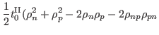
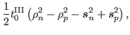
that includes zero-range class II and III forces.
We consider the following zero-range
interactions of class II and III with two new low-energy
coupling constants
-mixed DFT [16,19,20]
that includes zero-range class II and III forces.
We consider the following zero-range
interactions of class II and III with two new low-energy
coupling constants
![]() and
and
![]() [26]:
[26]:
Contributions of class III force to EDF (6) depend
on the standard nn and pp densities and,
therefore, can
be taken into account within the conventional ![]() -separable DFT
approach [9].
In contrast, contributions of class II force
(5) depend explicitly on the
mixed densities,
-separable DFT
approach [9].
In contrast, contributions of class II force
(5) depend explicitly on the
mixed densities, ![]() and
and
![]() , and require the use
of
, and require the use
of ![]() -mixed DFT [27,28], augmented by the isospin
cranking to control the magnitude and direction of the isospin
-mixed DFT [27,28], augmented by the isospin
cranking to control the magnitude and direction of the isospin ![]() .
.
We implemented the new terms of the EDF in the code
HFODD [19,20], where the isospin degree of freedom is
controlled within the isocranking method [29,30,27] - an
analogue of the cranking technique that is widely used in high-spin
physics. The isocranking method allows us to calculate the entire
isospin multiplet, ![]() , by starting from an isospin-aligned state
, by starting from an isospin-aligned state
![]() and isocranking it around the
and isocranking it around the ![]() -axis in the
isospace. The method can be regarded as an approximate isospin
projection. A rigorous treatment of the isospin symmetry
within the
-axis in the
isospace. The method can be regarded as an approximate isospin
projection. A rigorous treatment of the isospin symmetry
within the ![]() -mixed DFT formalism requires full, three-dimensional
isospin projection, which is currently under development.
-mixed DFT formalism requires full, three-dimensional
isospin projection, which is currently under development.
Physically relevant values of
![]() and
and
![]() turn out to be fairly
small [26], and thus the new terms do not impair the
overall agreement of self-consistent results with the standard
experimental data. Moreover, calculated MDEs and TDEs depend on
turn out to be fairly
small [26], and thus the new terms do not impair the
overall agreement of self-consistent results with the standard
experimental data. Moreover, calculated MDEs and TDEs depend on
![]() and
and
![]() almost linearly, and, in addition, MDEs (TDEs) depend very
weakly on
almost linearly, and, in addition, MDEs (TDEs) depend very
weakly on
![]() (
(
![]() ) [26]. This allows us to use the standard linear
regression method, see, e.g. Refs. [31,32], to
independently adjust
) [26]. This allows us to use the standard linear
regression method, see, e.g. Refs. [31,32], to
independently adjust
![]() and
and
![]() to experimental values of TDEs
and MDEs, respectively.
See Supplemental Material [21] for
detailed description of the procedure.
Coupling
constants
to experimental values of TDEs
and MDEs, respectively.
See Supplemental Material [21] for
detailed description of the procedure.
Coupling
constants
![]() and
and
![]() resulting from such an adjustment are
collected in Table 1.
resulting from such an adjustment are
collected in Table 1.
| SV |
SkM* | SLy4 | ||||
|
|
||||||
|
|
|
|
|
In Fig. 2, we show values of MDEs calculated within
our extended DFT formalism for the Skyrme SV![]() EDF. By
subtracting an overall linear trend (as defined in
Fig. 1) we are able to show results in extended
scale, where a detailed comparison with experimental data is
possible. In Fig. 3, we show results obtained for
TDEs, whereas complementary results obtained for the Skyrme SkM* and SLy4 EDFs
are collected in the Supplemental Material [21].
EDF. By
subtracting an overall linear trend (as defined in
Fig. 1) we are able to show results in extended
scale, where a detailed comparison with experimental data is
possible. In Fig. 3, we show results obtained for
TDEs, whereas complementary results obtained for the Skyrme SkM* and SLy4 EDFs
are collected in the Supplemental Material [21].
It is gratifying to see that the calculated values of MDEs closely
follow the experimental ![]() -dependence, see Fig. 2. It
is worth noting that
a single
coupling constant
-dependence, see Fig. 2. It
is worth noting that
a single
coupling constant
![]() reproduces
both
reproduces
both ![]() and
and ![]() MDEs, which confirms conclusions
of Ref. [9]. In addition, for the
MDEs, which confirms conclusions
of Ref. [9]. In addition, for the ![]() MDEs, the
SV
MDEs, the
SV![]() results nicely reproduce (i) changes in experimental
trend that occur at
results nicely reproduce (i) changes in experimental
trend that occur at ![]() and 39, (ii) staggering pattern between
and 39, (ii) staggering pattern between
![]() and 39, and (iii) disappearance of staggering between
and 39, and (iii) disappearance of staggering between ![]() and 49 (the f
and 49 (the f![]() nuclei). We note that these features are
already present in the SV
nuclei). We note that these features are
already present in the SV![]() results without the ISB terms,
and that adding this terms increases amplitude of the staggering.
However, for the SkM* and SLy4 functionals, the staggering of the
results without the ISB terms,
and that adding this terms increases amplitude of the staggering.
However, for the SkM* and SLy4 functionals, the staggering of the
![]() MDEs is less pronounced [21]. We also note that
all three functionals correctly describe the
MDEs is less pronounced [21]. We also note that
all three functionals correctly describe the ![]() -dependence and lack
of staggering of the
-dependence and lack
of staggering of the ![]() MDEs.
MDEs.
It is even more gratifying to see
in Fig. 3
that our ![]() -mixed calculations,
with
the class-II coupling constant,
-mixed calculations,
with
the class-II coupling constant,
![]() , describe absolute
values
as well as staggering of TDEs very well,
whereas results obtained without ISB terms give
too small values
and show no staggering. Good agreement obtained for the MDEs
and TDEs shows that the role and magnitude of the ISB terms
are
now firmly established.
, describe absolute
values
as well as staggering of TDEs very well,
whereas results obtained without ISB terms give
too small values
and show no staggering. Good agreement obtained for the MDEs
and TDEs shows that the role and magnitude of the ISB terms
are
now firmly established.
![\includegraphics[width=\columnwidth]{Figure02.eps}](img64.png) |
It is very instructive to look at ten outliers
which were excluded from the fitting procedure.
They are shown by open symbols
in Figs. 2 and 3.
(i) There are five outliers that
depend on masses of ![]() Co,
Co, ![]() Cu, and
Cu, and ![]() Rb,
which clearly deviate from the calculated trends for MDEs and TDEs.
These masses were not directly measured but
derived from systematics [24].
(ii) There are two
outliers that depend on the mass of
Rb,
which clearly deviate from the calculated trends for MDEs and TDEs.
These masses were not directly measured but
derived from systematics [24].
(ii) There are two
outliers that depend on the mass of ![]() V, whose ground-state
measurement may be contaminated by an unresolved
isomer [33,34,35].
(iii) Large differences between experimental and calculated values
are found in MDE for
V, whose ground-state
measurement may be contaminated by an unresolved
isomer [33,34,35].
(iii) Large differences between experimental and calculated values
are found in MDE for ![]() , 67 and 69.
Inclusion of these data in the fitting procedure would significantly
increase the uncertainty of adjusted coupling constants.
The former two,
(i) and (ii),
call for improving experimental values,
whereas the last one (iii) may be a result of structural effects not
included in our model.
, 67 and 69.
Inclusion of these data in the fitting procedure would significantly
increase the uncertainty of adjusted coupling constants.
The former two,
(i) and (ii),
call for improving experimental values,
whereas the last one (iii) may be a result of structural effects not
included in our model.
Having at hand a model with ISB strong interactions with fitted
parameters we can calculate MDEs for more massive multiplets and make
predictions on binding energies of neutron-deficient (![]() )
nuclei.
In particular,
in Table 2 we present predictions of mass excesses
of
)
nuclei.
In particular,
in Table 2 we present predictions of mass excesses
of ![]() Co,
Co, ![]() Cu, and
Cu, and ![]() Rb, whose masses were in
AME12 [24] derived from systematics, and
Rb, whose masses were in
AME12 [24] derived from systematics, and ![]() V, whose
ground-state mass measurement is uncertain. Recently, the mass excess
of
V, whose
ground-state mass measurement is uncertain. Recently, the mass excess
of ![]() Co was measured as
Co was measured as ![]() 34361(8) [36] or
34361(8) [36] or
![]() 34331.6(66) keV [37]. These values are in fair agreement
with our prediction (1.8 or 2.4
34331.6(66) keV [37]. These values are in fair agreement
with our prediction (1.8 or 2.4![]() difference with respect to
our estimated theoretical uncertainty), even though the difference
between them is still far beyond the estimated (much smaller)
experimental uncertainties.
difference with respect to
our estimated theoretical uncertainty), even though the difference
between them is still far beyond the estimated (much smaller)
experimental uncertainties.
| Mass excess (keV) | ||||
| Nucleus | This work | AME12 [24] | ||
![\includegraphics[width=\columnwidth]{Figure04.eps}](img70.png) |
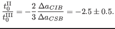
Assuming that the extracted CSB and CIB effects are, predominantly,
due to the ISB in the ![]() channel we can relate ratio
channel we can relate ratio
![]() /
/
![]() to the experimental scattering lengths. The reasoning follows
the work of Suzuki et al. [10], which assumed a
proportionality between the strengths of CSB and CIB forces and
the corresponding scattering lengths [38], that is,
to the experimental scattering lengths. The reasoning follows
the work of Suzuki et al. [10], which assumed a
proportionality between the strengths of CSB and CIB forces and
the corresponding scattering lengths [38], that is,
![]() and
and
![]() , which, in our case, is
equivalent to
, which, in our case, is
equivalent to
![]() and
and
![]() . Assuming further that
the proportionality constant is the same, and taking for the
experimental values
. Assuming further that
the proportionality constant is the same, and taking for the
experimental values
![]() and
and
![]() [38], one gets:
[38], one gets:
In summary, we showed that the ![]() -mixed DFT with added two new terms related to
the ISB interactions of class II and III is able to systematically
reproduce observed MDEs and TDEs of
-mixed DFT with added two new terms related to
the ISB interactions of class II and III is able to systematically
reproduce observed MDEs and TDEs of ![]() and
and ![]() multiplets.
Adjusting only two coupling constants
multiplets.
Adjusting only two coupling constants
![]() and
and
![]() , we reproduced
not only the magnitudes of the MDE and TDE but also
their characteristic staggering patterns.
The obtained values of
, we reproduced
not only the magnitudes of the MDE and TDE but also
their characteristic staggering patterns.
The obtained values of
![]() and
and
![]() turn out to agree with the
turn out to agree with the ![]() ISB interactions (
ISB interactions (![]() scattering lengths) in the
scattering lengths) in the ![]() channel.
We predicted mass excesses of
channel.
We predicted mass excesses of ![]() Co,
Co, ![]() Cu,
Cu, ![]() Rb, and
Rb, and
![]() V, and for
V, and for ![]() Co we obtained fair agreement with
the recently measured values [36,37]. To better pin down
the ISB effects, accurate mass measurements of the other three nuclei
are very much called for.
Co we obtained fair agreement with
the recently measured values [36,37]. To better pin down
the ISB effects, accurate mass measurements of the other three nuclei
are very much called for.
This work was supported in part by the Polish National Science Center under Contract Nos. 2014/15/N/ST2/03454 and 2015/17/N/ST2/04025, by the Academy of Finland and University of Jyväskylä within the FIDIPRO program, by Interdisciplinary Computational Science Program in CCS, University of Tsukuba, and by ImPACT Program of Council for Science, Technology and Innovation (Cabinet Office, Government of Japan). We acknowledge the CIS Swierk Computing Center, Poland, and the CSC-IT Center for Science Ltd., Finland, for the allocation of computational resources.
![\includegraphics[width=\columnwidth]{Figure03.eps}](img65.png)