Next: Densities in the spherical
Up: The NLO potentials, fields,
Previous: The NLO potentials, fields,
Spherical HO basis
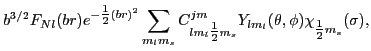
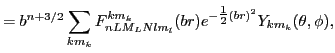
The standard spherical HO wave functions, are given by
where  is the oscillator constant,
 |
|
|
(79) |
and  are proportional to the standard Laguerre polynomials [7].
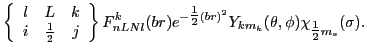
To calculate the secondary densities (76), one has to
act on the space part of the wave function (79) with the
derivative operators  . This leads to defining the
polynomials
. This leads to defining the
polynomials
 such that
| |
|
 |
|
| |
|
 |
(80) |
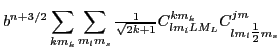
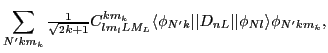
where 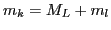 . From the Wigner-Eckart theorem, these polynomials
must have the form:
. From the Wigner-Eckart theorem, these polynomials
must have the form:
and our goal is to determine the set of reduced polynomials
 ,
in terms of which the derivatives of the spherical HO wave functions read
,
in terms of which the derivatives of the spherical HO wave functions read
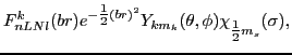
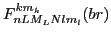
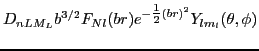
Explicit form of
can be calculated by using the
Wigner-Eckart theorem again, namely, Eq. (81) must have the
form
where  is the space part of the wave function (79).
Then we have polynomials
expressed through the Laguerre
polynomials as:
is the space part of the wave function (79).
Then we have polynomials
expressed through the Laguerre
polynomials as:
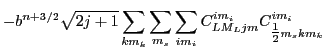
where the reduced matrix element can be calculated by considering
only one matrix element, namely,
Note that the Clebsh-Gordan coefficient  is not
zero for angular momenta restricted by the parity conservation,
is not
zero for angular momenta restricted by the parity conservation,
 .
.
The parity conservation induces specific conditions on the polynomials
.
Indeed, by comparing parities of both sides of Eq. (81) we see
that
Equivalently, since for all derivative operators we have  , we see that
Since polynomials  are real, phases of polynomials
are fixed by those of the derivative operators
(31) and spherical harmonics [6],
are real, phases of polynomials
are fixed by those of the derivative operators
(31) and spherical harmonics [6],
that is,
where the last two equivalent forms result from Eqs (87) and (88).
The  polynomials are calculated using formulas for spherical
derivatives (see [6] ) combined with recursion relations
for derivatives of Laguerre polynomials. In this way
spherical derivatives of one of the basis functions
polynomials are calculated using formulas for spherical
derivatives (see [6] ) combined with recursion relations
for derivatives of Laguerre polynomials. In this way
spherical derivatives of one of the basis functions
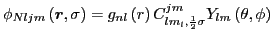 can be expressed as a sum of functions
where the  and coefficients needed for the different orders were derived
using symbolic programming. In this way we obtain analytical expressions for
all derivatives which can then be calculated with good accuracy.
and coefficients needed for the different orders were derived
using symbolic programming. In this way we obtain analytical expressions for
all derivatives which can then be calculated with good accuracy.
Next: Densities in the spherical
Up: The NLO potentials, fields,
Previous: The NLO potentials, fields,
Jacek Dobaczewski
2010-01-30
![\begin{eqnarray*}
\nabla_{1\mu_{1}}..\nabla_{1\mu_{N}}g_{nl}\left(r\right)Y_{lm}...
...}\left(r\right)\right]Y_{l+i_{1}+..+i_{n},m+\mu_{1}+..+\mu_{N}},
\end{eqnarray*}](img269.png)