Next: Fields for terms containing
Up: General forms of the
Previous: Potentials
Fields
Now we are in a position to perform the variation of densities
over the wave functions. To this end, we assume that
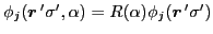
the non-local density matrices in Eq. (40)
have the general form of
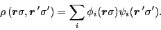 |
(46) |
This form allows us to carry out the derivation for several
important specific cases simultaneously. Namely, for
the standard HF case one has:
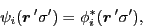 |
(47) |
and the sum runs over the occupied states only,  .
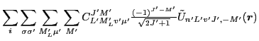
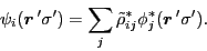
Similarly, for the BCS case, or for the HFB case in the canonical basis, one has:
.
Similarly, for the BCS case, or for the HFB case in the canonical basis, one has:
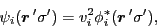 |
(48) |
where  are the occupation factors and the sum runs over
the pairing window. For transition densities pertaining to the
symmetry restoration, one has:
are the occupation factors and the sum runs over
the pairing window. For transition densities pertaining to the
symmetry restoration, one has:
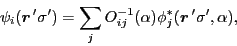 |
(49) |
Where
 are the wave functions transformed by the symmetry operator
  and
and
 is the overlap matrix:
 |
(50) |
Finally, for the RPA amplitudes given by non-hermitian matrix
 one has
 |
(51) |
To derive the fields,
first we recall that the variation of the non-local density,
over the wave function reads
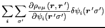
Therefore, variation of the primary density is given by
At this point, operators  mix derivatives acting on
the variables
mix derivatives acting on
the variables  and
and  , cf. Eq. (18).
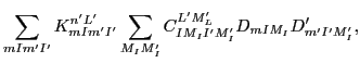
By using the Wigner-Eckart theorem, we can express them as sums of
products of derivatives
, cf. Eq. (18).
By using the Wigner-Eckart theorem, we can express them as sums of
products of derivatives  and
and  , which act
on and , respectively, that is,
, which act
on and , respectively, that is,
where the order of derivative is conserved,
 |
|
|
(55) |
and the triangle rule
of angular momentum coupling must be obeyed. Numerical coefficients
 can be calculated by using methods of symbolic programming.
At N
can be calculated by using methods of symbolic programming.
At N LO, only 91 coefficients
are needed,
so they can easily be precalculated and stored.
LO, only 91 coefficients
are needed,
so they can easily be precalculated and stored.
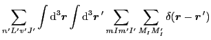
We now can insert expressions (54) and
(55) into Eq. (45)
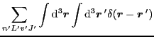
and remove condition
 by adding the integral
over and the function
by adding the integral
over and the function
 , that is,
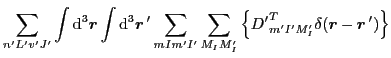
This allows us to integrate by parts over
and transfer the action of onto the delta function.
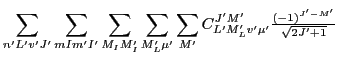
With all the angular momenta couplings shown explicitly, this gives
The action of
 onto the delta function can be replaced
by that of
onto the delta function can be replaced
by that of
 , and then the integration by parts
over gives,
, and then the integration by parts
over gives,
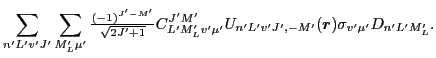
In the resulting local integral
we request that the operator acting on
 is equal to the mean-field operator, which gives
In this form, the mean-field operator is expressed through sums of derivative
operators standing on both sides of the potentials
 . This form
can easily be used in the calculation of the matrix elements, because
the left derivative operator can simply be applied onto the
left wave-function through the integration by parts.
Moreover, potentials
are related to the
secondary densities by very simple relations (46).
However, it turns
out that numerical calculations are much faster if the
derivatives appear only on one side of the potentials, like it was postulated
in Eq. (7), that is,
. This form
can easily be used in the calculation of the matrix elements, because
the left derivative operator can simply be applied onto the
left wave-function through the integration by parts.
Moreover, potentials
are related to the
secondary densities by very simple relations (46).
However, it turns
out that numerical calculations are much faster if the
derivatives appear only on one side of the potentials, like it was postulated
in Eq. (7), that is,
Next: Fields for terms containing
Up: General forms of the
Previous: Potentials
Jacek Dobaczewski
2010-01-30