Conventional Skyrme EDF
can be expressed by bilinear forms of six isoscalar (![]() )
and six isovector (
)
and six isovector (![]() ) local densities, including the particle
) local densities, including the particle ![]() ,
kinetic
,
kinetic ![]() , spin
, spin ![]() , spin-kinetic
, spin-kinetic ![]() , current
, current ![]() ,
and spin-current
,
and spin-current
![]() densities and
their derivatives. Standard definitions of these densities can be found in numerous
references, see, e.g., Refs. [9,46] and references quoted therein.
It is to be noted that in the standard MF
theory the proton and neutron s.p. wave functions are not mixed, i.e., the proton-neutron symmetry is strictly conserved [46,47].
Therefore, the MF isoscalar (isovector) densities are
simply sums (differences) of neutron and proton densities since only the third component of the isovector density
is nonzero.
densities and
their derivatives. Standard definitions of these densities can be found in numerous
references, see, e.g., Refs. [9,46] and references quoted therein.
It is to be noted that in the standard MF
theory the proton and neutron s.p. wave functions are not mixed, i.e., the proton-neutron symmetry is strictly conserved [46,47].
Therefore, the MF isoscalar (isovector) densities are
simply sums (differences) of neutron and proton densities since only the third component of the isovector density
is nonzero.
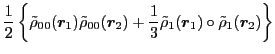
The isospin projection essentially preserves the functional form of the Skyrme EDF derived by
averaging the isospin-invariant Skyrme interaction over the Slater determinant.
All what needs to be done is a replacement of the local density matrix by the
corresponding transition density matrix. Moreover, the
bilinear terms that depend of the isovector densities must be
replaced by the full isoscalar products of the corresponding
isovector transition densities.
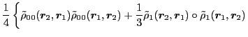
Special care should be taken of the density-dependent term of the Skyrme
interaction as the extension of this term
to the transition case
is undefined in the process of
averaging the Skyrme interaction over the Slater determinant. Following the argumentation of
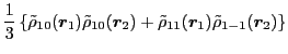
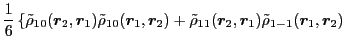
Refs. [48,49], we replace the isoscalar density by the
transition isoscalar density matrix, that is,
![]() .
.
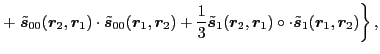
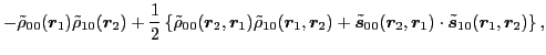
As for the Coulomb-interaction kernel, it depends on the isoscalar
and isovector transition densities in the following way:
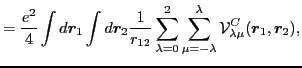 |
(52) |