Fitting the tensor strengths to single-particle energies

Figure 1: The $\pi h_{11/2}-\pi g_{7/2}$ splitting in $_{51}^A$Sn isotopes versus $A$. Black triangles label empirical data taken from Ref. [18]. Open and gray symbols represent the SHF results obtained by using the SLy4 (left) SkO (middle), and SLy5 (right) parameterizations, respectively. Different symbols labeling theoretical results follow the SHF minima corresponding to configurations differing in the $\nu h_{11/2}$ occupancies as indicated in the legend.

The s.p. levels constitute one of the main building blocks of the MF method. In spite of that, the Skyrme HF (SHF) method that uses forces fitted to bulk nuclear properties performs rather poorly with regard to the s.p. SO splittings[28,30]. This is visualized in Fig. 1, showing the $\pi 1h_{11/2}-\pi 1g_{7/2}$ splittings, $\Delta E_{gh}$, in antimony, calculated by using the SLy4[35], SkO[36], and SLy5[35] parameterizations. The SLy4 force strongly overestimates the absolute value of $\Delta E_{gh}$ and fails to reproduce the slope of the $\Delta E_{gh} (A)$ curve. The non-standard isovector SO in the SkO force helps by reducing, on average, the splitting to the empirical level, but does not change the slope of the $\Delta E_{gh} (A)$ curve. Finally, in SLy5, the inclusion of tensor terms changes the slope, but shifts the theoretical curves in a wrong direction. The latter observation suggests that the fit to masses leads to values of tensor coupling constants that are at variance with those deduced from the s.p. level analysis, see Refs.[37,28]. However, one should point out that the $\pi 1h_{11/2}-\pi 1g_{7/2}$ splittings depend upon many factors including, apart from the SO and tensor fields, the effective mass, centroid energies of the $\ell = 4$ and $\ell = 5$ sub-shells, and strong polarization effects. Hence, conclusions concerning the SO and tensor coupling constants that are deduced solely from these data should be considered to be tentative.

Figure 2: The neutron (top) and proton (bottom) $1f_{7/2}-1f_{5/2}$ SO splittings in $^{40}$Ca, $^{48}$Ca, and $^{56}$Ni. Black symbols show the mean empirical values taken from Refs.[38,39] and open dots denote the SkO results. Open diamonds represent the results obtained by using the SkO$_{T^\prime}$ functional of Ref.[40], which includes strong attractive tensor terms and a reduced SO strength.

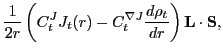
It is well known, see Refs.[41,42], that the tensor interaction strongly modifies the SO one-body potential. In the spherical-symmetry limit, the isoscalar ($t=0$) and isovector ($t=1$) SO one-body potentials read:

$$W_t^{SO} = \frac{1}{2r}\left( C^J_t J_t(r) - C^{\nabla J}_t \frac{d\rho_t}{dr}\right) {\mathbf L} \cdot {\mathbf S},$$ (1)

where $C^J_t$ and $C^{\nabla J}_t$ are the tensorial and spin-orbit coupling constants, see for example Ref.[28]. The tensor field depends upon the radial component of the spin-orbit vector density ${\mathbf J}_t=\frac{{\mathbf r}}{r}J_t(r)$ that measures the spin-asymmetry of the nucleus and can rapidly vary with particle numbers. On the contrary, the second term in Eq. (1), which is due to the conventional two-body spin-orbit interaction, depends on the radial derivative of the particle density $\rho_t$, which varies relatively slowly with particle numbers. Such a contrasting behavior of the two major constituents of the SO potential can be actually used to fit the coupling constants to data[28]. The idea is visualized in Fig. 2, which shows the $1f_{7/2}-1f_{5/2}$ SO splittings in $^{40}$Ca, $^{48}$Ca, and $^{56}$Ni. These splittings form a very distinct pattern that cannot be reproduced based solely on the conventional SO potential. Indeed, the $1f_{7/2}-1f_{5/2}$ SO splittings in $^{40}$Ca, $^{48}$Ca, and $^{56}$Ni are fairly constant when calculated using, for example the SkO force, see curve marked by open dots in Fig. 2. It reflects the fact that the neutron and proton radial form-factors $\frac{d\rho}{dr}$ almost do not change when going from $^{40}$Ca through $^{48}$Ca to $^{56}$Ni. At the same time the neutron and proton SO vector densities $J(r)$ change rapidly when going from the isoscalar spin-saturated $^{40}$Ca to the isoscalar spin-unsaturated nucleus $^{56}$Ni, and, finally, to the isovector spin-unsaturated nucleus $^{48}$Ca. This allows for a simple and intuitive three-step fitting procedure[28] of the $C^{\nabla J}_0$ in $^{40}$Ca, $C^{J}_0$ in $^{56}$Ni, and $C^{J}_1/ C^{\nabla J}_1$ ratio in $^{48}$Ca. This procedure leads to (i) a significant reduction in the isoscalar SO strength and (ii) strong attractive tensor coupling constants. It systematically improves such s.p. properties as the SO splittings and magic-gap energies[28], but leads to deteriorated nuclear binding energies.