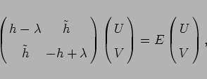
By varying the energy functional (3) with respect to the
density matrices ![]() and
and
![]() one arrives at the HFB equations:
one arrives at the HFB equations:
The HFB equations (6), also called the Bogoliubov de Gennes equations by condensed matter physicists, are the generalized Kohn Sham equations of the DFT. It is worth noting that - in its original formulation [15] - the DFT formalism implicitly includes the full correlation functional. In most nuclear applications, however, the correlation corrections are added afterwards. Those corrections usually include the following terms: the center-of-mass correction, rotational correction associated with the spontaneous breaking of rotational symmetry, vibrational correction (quantum zero-point vibrational fluctuations), particle-number correction due to the broken gauge invariance, as well as other terms.
The spectrum of quasi-particle energies ![]() is continuous for
is continuous for
![]()
![]()
![]() and discrete for
and discrete for ![]()
![]()
![]() .
However, when
solving the HFB equations on a coordinate-space lattice of points
or by expanding quasi-particle
wave functions in a finite basis, the quasi-particle spectrum
is discretized and one can use the notation
.
However, when
solving the HFB equations on a coordinate-space lattice of points
or by expanding quasi-particle
wave functions in a finite basis, the quasi-particle spectrum
is discretized and one can use the notation
![]() and
and
![]() .
Since for
.
Since for ![]()
![]() 0 and
0 and ![]()
![]() 0 the lower
components
0 the lower
components
![]() are localized functions of
are localized functions of
![]() ,
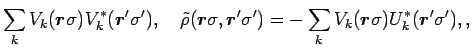
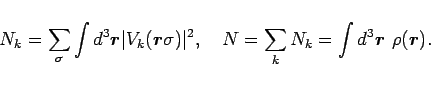
the density matrices,
,
the density matrices,
For spherical nuclei, the self-consistent HFB equations are best solved in the coordinate space where they form a set of 1D radial differential equations [16,17]. In the case of deformed nuclei, however, the solution of deformed HFB equations in coordinate space is a difficult and time-consuming task. For axial nuclei, the corresponding 2D differential equations can be solved by using the basis-spline methods (see, e.g., Ref. [18]). For triaxial nuclei, 3D solutions in a restricted space are possible by using the so-called two-basis method [19].