


Next: HFB sum rules
Up: Particle-Number-Projected HFB
Previous: Shifted HFB states
Projected HFB states
The Thouless theorem (7) allows us to express the HFB
state  and shifted HFB state
 as sums of components having different particle numbers,
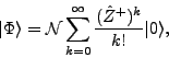 |
(11) |
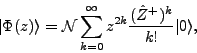 |
(12) |
where
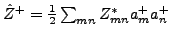 is the
Thouless pair-creation operator.
It then trivially follows that the
shift transformation does not change any of the
particle-number-projected states (2),
is the
Thouless pair-creation operator.
It then trivially follows that the
shift transformation does not change any of the
particle-number-projected states (2),
 |
(13) |
but only scales the coefficients in the sum of Eq. (12).
Since the shifted states
(12) are manifestly analytical in  , all closed contours
  in Eq. (2)
give, by the Cauchy theorem, the same result.
Among them, the integral in Eq. (1) simply
corresponds to the unit circle.
in Eq. (2)
give, by the Cauchy theorem, the same result.
Among them, the integral in Eq. (1) simply
corresponds to the unit circle.
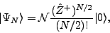
The analyticity of
results in a simple and
elegant representation of the projected state:
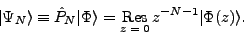 |
(14) |
Indeed, in the sum of Eq. (12), only the term with  particles is multiplied by
  and thus contributes to the
residue at
and thus contributes to the
residue at  . This observation allowed Dietrich, Mang, and Pradal
[36] to formulate the so-called method of residues
for calculating all kinds of matrix elements involving the
projected state
. This observation allowed Dietrich, Mang, and Pradal
[36] to formulate the so-called method of residues
for calculating all kinds of matrix elements involving the
projected state
 . For example, the average HFB energy
of the projected state can be written as a ratio of two residues:
. For example, the average HFB energy
of the projected state can be written as a ratio of two residues:
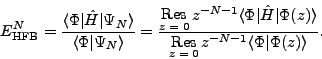 |
(15) |
The invariance of the projected state with respect to the integration
contour can be formulated in another way; namely, one can utilize the
property that an arbitrarily shifted HFB state can be equally well used
to project the particle number. Indeed, for
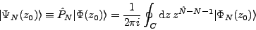 |
(16) |
we trivially have
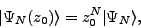 |
(17) |
i.e., projection from a shifted HFB state changes only the phase and
normalization of the projected state. We refer to this property as
shift invariance.
Next: HFB sum rules
Up: Particle-Number-Projected HFB
Previous: Shifted HFB states
Jacek Dobaczewski
2007-08-08