


Next: Calculation of matrix elements
Up: Interaction matrix elements (second
Previous: Interaction matrix elements (second
In this appendix, we discuss interaction matrix elements coming from
![$E[\rho,\kappa,\kappa^\ast]$](img137.png) ,
which we take to contain separate Skyrme (i.e. strong-force,
,
which we take to contain separate Skyrme (i.e. strong-force,
 -independent), Coulomb, and pairing energy functionals:
![\begin{displaymath}
E[\rho,\kappa,\kappa^\ast]
= E_{\rm Skyrme}[\rho] + E_{\rm Coul}[\rho_{\rm p}] +E_{\rm pair}[\rho,\kappa,\kappa^\ast],
\end{displaymath}](img195.png) |
(25) |
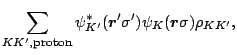
where  is the proton density matrix.
The most general Skyrme energy functional in common use is given by
is the proton density matrix.
The most general Skyrme energy functional in common use is given by
(See, e.g., [79,80,63] and references therein for a general
discussion.)
All densities are labeled by isospin indices  , where
  takes values zero and one and
  is always equal to 0.
A more general theory could violate isospin at the single-quasiparticle level,
leading to additional densities
is always equal to 0.
A more general theory could violate isospin at the single-quasiparticle level,
leading to additional densities  [63].
We do not consider such densities here.
The
[63].
We do not consider such densities here.
The  are the coupling constants for the effective interaction.
As usual, two of them are chosen to be density dependent:
are the coupling constants for the effective interaction.
As usual, two of them are chosen to be density dependent:
Here  ,
,
 ,
,  ,
,
 ,
,
 ,
,
 , and
, and
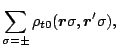
 are local densities and currents, which
are derived from the general density matrices for protons and neutrons
are local densities and currents, which
are derived from the general density matrices for protons and neutrons
where
and
 labels the spin components so that, e.g.,
 is a spin component of the single-particle wave
function associated with the state
is a spin component of the single-particle wave
function associated with the state
 .
Defining
.
Defining
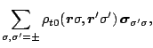
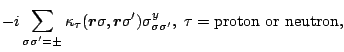
where
 is a matrix element of the vector of
Pauli spin matrices, we write the local densities and currents as
is a matrix element of the vector of
Pauli spin matrices, we write the local densities and currents as
The Coulomb energy functional is given by
![\begin{displaymath}
E_{\mbox{\footnotesize {Coul}}} [\rho_{\rm p}]
= \frac{e^2}{...
...{\footnotesize {p}}}^{4/3} (\mbox{\boldmath$r$\unboldmath })
,
\end{displaymath}](img245.png) |
(32) |
where we make the usual Slater approximation [81] for the exchange term.
For the pairing functional we take the quite general form
![\begin{displaymath}
E_{\mbox{\footnotesize {pair}}}[\rho,\kappa,\kappa^\ast]
= E...
...ert\tilde{\rho}_\tau(\mbox{\boldmath$r$\unboldmath })\vert^2 ,
\end{displaymath}](img246.png) |
(33) |
where the density-dependent pairing coupling constant
![$C^{\tilde\rho}[\rho_{00}(\mbox{\boldmath$r$\unboldmath })]$](img247.png) is an arbitrary function of
is an arbitrary function of
 .
The quantity
.
The quantity
 is defined as [64]
with
being the standard pairing tensor in the coordinate representation.
The second derivatives of the energy functional in Eq. (13), as the equation indicates and we've
already noted, can be written
as unsymmetrized matrix elements
 of an effective interaction between uncoupled pairs of single-particle
states. The particle-hole matrix elements take the form
of an effective interaction between uncoupled pairs of single-particle
states. The particle-hole matrix elements take the form
 |
(36) |
The last term contains the pairing rearrangement discussed at the end of the
previous appendix.
The effective Skyrme interaction in Eq. (37) is given by
 is the vector of
Pauli matrices in isospin space and
is the vector of
Pauli matrices in isospin space and
The coefficients in Eq. (38) are defined in
Tables 3 and 4.
Equation (38) contains the usual
Skyrme-interaction operators,
but, the energy functional (27) does not necessarily correspond
to a real (density-dependent) two-body Skyrme interaction because the
matrix elements
are not antisymmetrized.
Compared to the case usually discussed in the literature, the more general
functional relaxes relations that would otherwise restrict the spin-isospin structure of
the effective interaction
in Eq. (38); see, e.g., [16]
for a discussion of the increased freedom.
The densities and currents that appear in Eq. (38)
come mostly from rearrangement terms and take
the values given by the HFB ground state.
The isoscalar and isovector spin densities
 vanish when the
HFB ground state is time-reversal invariant or spherical as assumed here.
The terms containing them will therefore not appear in the expressions for the matrix elements
of the effective interaction for such states given below.
vanish when the
HFB ground state is time-reversal invariant or spherical as assumed here.
The terms containing them will therefore not appear in the expressions for the matrix elements
of the effective interaction for such states given below.
Table 3:
Definitions of

 ,
,  , and
, and  in Eq. (38).
 |
 |
 |
 |
 |
| 0 |
 |
 |
 |
 |
| 1 |
 |
 |
 |
 |
| 2 |
 |
 |
 |
 |
| 3 |
 |
 |
 |
 |
| 4 |
 |
|
 |
|
Table 4:
Definitions
of the coefficients appearing in the rearrangement terms
in Eq. (38).
|
 |
 |
 |
 |
 |
 |
| 3 |
 |
 |
 |
 |
 |
 |
The effective Coulomb interaction in Eq. (37), acting between
protons, is given by
 |
(39) |
Finally, the ph-type pairing-rearrangement terms in Eq. (37) come
from an effective interaction
 |
(40) |
The second derivatives with respect to
 also can be
written as unsymmetrized matrix elements of effective interactions, this time
in the particle-particle channel. The particle-particle effective interaction entering the matrix elements
also can be
written as unsymmetrized matrix elements of effective interactions, this time
in the particle-particle channel. The particle-particle effective interaction entering the matrix elements
 |
(41) |
is obtained from Eq. (34)
through Eq. (14) as
 |
(42) |
In the numerical calculations of this paper, we use a volume pairing-energy functional,
i.e.,
 |
(43) |
Last of all are the mixed functional derivatives involving both  and
(or
and
(or  )
in Eq. (15). They also can be
written as the unsymmetrized matrix elements of an effective interaction:
)
in Eq. (15). They also can be
written as the unsymmetrized matrix elements of an effective interaction:
 |
(44) |
where  denotes the time-reversed state of , and the
3p1h effective interaction itself is
denotes the time-reversed state of , and the
3p1h effective interaction itself is
 |
(45) |
where  acts on the single-particle states
  and in
Eq. (45), and the eigenvalues 1 and
and in
Eq. (45), and the eigenvalues 1 and  are
assigned to the neutron and proton, respectively.
are
assigned to the neutron and proton, respectively.
Next: Calculation of matrix elements
Up: Interaction matrix elements (second
Previous: Interaction matrix elements (second
Jacek Dobaczewski
2004-07-29

![$\displaystyle \sum_{t=0,1} \int d^3r
\bigg\{ C_t^{\rho}[\rho_{00}]\, \rho^2_{t0...
...\mbox{\boldmath$j$\unboldmath }^2_{t0}(\mbox{\boldmath$r$\unboldmath })
\right]$](img198.png)
![$\displaystyle + C_t^{\nabla J}
\left[ \rho_{t0}(\mbox{\boldmath$r$\unboldmath }...
...oldmath$j$\unboldmath }_{t0}(\mbox{\boldmath$r$\unboldmath })
\right]
\bigg\} .$](img200.png)