Theory

The isospin-projected DFT technique [11,12,13] utilizes the ability of the self-consistent MF method to properly describe the balance between the long-range Coulomb force and the short-range nuclear interaction, represented in this work by the Skyrme-type energy density functional (EDF). To remove the spurious isospin-symmetry-breaking effects, we use the standard one-dimensional isospin projection after variation, which allows us to decompose the Slater determinant $\vert\Phi\rangle$ into good isospin states $\vert T,T_z\rangle$:

$$\vert\Phi \rangle = \sum_{T\geq \vert T_z\vert}b_{T,T_z}\ver... ... \quad \sum_{T\geq \vert T_z\vert} \vert b_{T,T_z}\vert^2 = 1.$$ (1)

Here, $\hat{P}^T_{T_z T_z}$ stands for the conventional one-dimensional isospin-projection operator:

$$\vert TT_z\rangle = \frac{1}{\sqrt{N_{TT_z}}}\hat{P}^T_{T_z T_z} \vert\Phi\rangle$$

$$= \frac{2T+1}{2 \sqrt{N_{TT_z}}}\int_0^\pi d\beta_T\; \sin\beta_T \; d^{T}_{T_z T_z}(\beta_T )\; \hat{R}(\beta_T )\vert\Phi\rangle ,$$ (2)

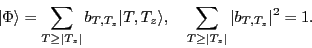
where $\beta_T$ denotes the Euler angle associated with the rotation operator $\hat{R}(\beta_T )= e^{-i\beta_T \hat{T}_y}$ about the $y$-axis in the isospace, $d^{T}_{T_z T_z}(\beta_T )$ is the Wigner function [17], and $T_z =(N-Z)/2$ is the third component of the total isospin $T$. The normalization factors $N_{TT_z}$, or interchangeably the expansion coefficients $b_{T,T_z}$ that encode the isospin content of $\vert\Phi\rangle$, read:

$$N_{T T_z} \equiv \vert b_{T,T_z}\vert^2 = \langle \Phi \vert \hat{P}^T_{T_z T_z} \vert \Phi \rangle$$

$$= \frac{2T+1}{2}\int_0^\pi d\beta_T \sin\beta_T \; d^{T}_{T_z T_z} (\beta_T ) \; {\mathcal N}(\beta_T),$$ (3)

where ${\mathcal N}(\beta_T) = \langle \Phi\vert \hat{R}(\beta_T)\vert \Phi\rangle$ is the so-called overlap kernel. For technical aspects concerning the calculation of the overlap and Hamiltonian kernels, we refer the reader to Ref. [13]. The isospin-projected DFT technique utilizes the ability of the HF solver HFODD [18] to produce fully symmetry-unrestricted Slater determinants $\vert\Phi\rangle$.

The isospin projection determines the set of good isospin states (called the basis in the following), which in the next step is used to rediagonalize the entire nuclear Hamiltonian, consisting of the kinetic energy, Skyrme EDF, and the isospin-breaking Coulomb force. The rediagonalization leads to the eigenstates:

$$\vert n,T_z\rangle = \sum_{T\geq \vert T_z\vert}a^n_{T,T_z}\vert T,T_z\rangle ,$$ (4)

numbered by index $n$. The amplitudes $a^n_{T,T_z}$ define the degree of isospin mixing through the so-called isospin-mixing coefficients (or isospin impurities) for the $n-$th eigenstate:

$$\alpha_C^n = 1 - \vert a^n_{T,T_z}\vert _{\mbox{\scriptsize {max}}}^2,$$ (5)

where $\vert a^n_{T,T_z}\vert _{\mbox{\scriptsize {max}}}^2$ stands for the squared norm of the dominant amplitude in the wave function $\vert n,T_z\rangle$. It is worth stressing that the isospin projection, unlike particle-number or angular-momentum projections, is essentially non-singular; hence, it can be safely used with the local EDFs. The rigorous analytical proof of this useful property can be found in Ref. [13].

The combined isospin and angular-momentum projection leads to the set of states,

$$\vert I,M,K; T,T_z\rangle = \frac{1}{\sqrt{N_{TT_z;IMK}}} \hat P^T_{T_z T_z} \hat P^I_{MK} \vert\Phi \rangle ,$$ (6)

which form another normalized basis built on $\vert\Phi\rangle$. Here, $\hat P^T_{T_z T_z}$ and $\hat P^I_{MK}$ stand for the isospin and angular-momentum projection operators, respectively, and $M$ and $K$ denote the angular-momentum components along the laboratory and intrinsic $z$-axes, respectively [19]. Now the problem becomes more complicated because of the overcompleteness of the basis (6) related to the $K$-mixing. This is overcome by performing the rediagonalization of the Hamiltonian in the so-called collective space, spanned for each $I$ and $T$ by the natural states, $\vert IM;TT_z\rangle^{(i)}$, as described in Refs. [18,20]. Such a rediagonalization gives the solutions:

$$\vert n; IM; T_z\rangle = \sum_{i,T\geq \vert T_z\vert} a^{(n)}_{iIT} \vert IM; TT_z\rangle^{(i)} ,$$ (7)

which are labeled by the index $n$ and by the conserved quantum numbers $I$, $M$, and $T_z =(N-Z)/2$ [cf. Eq. (4)].