Ab Initio Derivation of Model Energy Density Functionals

Jacek Dobaczewski

Abstract:

I propose a simple and manageable method that allows for deriving coupling constants of model energy density functionals (EDFs) directly from ab initio calculations performed for finite fermion systems. A proof-of-principle application allows for linking properties of finite nuclei, determined by using the nuclear nonlocal Gogny functional, to the coupling constants of the quasilocal Skyrme functional. The method does not rely on properties of infinite fermion systems but on the ab initio calculations in finite systems. It also allows for quantifying merits of different model EDFs in describing the ab initio results.

Approaches based on the density functional theory (DFT) provide us with very efficient and useful tools to describe properties of many-fermion systems like molecules, solids, or nuclei [1,2,3,4]. The range of possible various applications and implementations is extremely wide. In electronic systems, there exist numerous methods and techniques of linking the density functionals to the underlying Coulomb interaction, but in nuclei such links are much more difficult to explore, primarily because of the fact that nucleon-nucleon interactions are less obviously definable.

Only fairly recently, families of interactions based on chiral effective field theory [5,6,7,8,9,10,11] have become a gold standard for ab initio calculations of nuclear properties [12,13,14,15,16,17,18,19]. Based on this developments, there were already many attempts to link the nuclear DFT to these ab initio approaches [20,21,22,23,24,25,26,27]. Up to now, most of them referred directly (or indirectly, through the so-called density-matrix expansion (DME) [28]) to infinite-nuclear-matter properties. In this paper, I propose a generic method that directly links the ab initio approaches to the DFT in finite fermion systems.

A classic formulation of the DFT relies on a variational approach to the many-body problem, whereby it assumed that we are able to perform an exact variation of the average energy $\delta{E}=\delta\langle\Psi\vert\hat{H}\vert\Psi\rangle=0$, which gives us the exact ground-state energy $E_0$ and the exact ground-state wave-function $\vert\Psi_0\rangle$. By replacing the full variation with a two-stage variation, the DFT then appears in a very natural way.

The first-stage variation is performed under the constraint that the one-body local density of the system, $\rho(\bm{r})=\langle\Psi\vert a^+_{\bm{r}}a_{\bm{r}}\vert\Psi\rangle$, is fixed to a given density profile. Performing such a variation for all density profiles, one obtains the exact energy density functional (EDF) $E\left[\rho\right]$. In principle, such a constrained variation can be realized by an unconstrained variation performed for the system placed in an external one-body local potential $-U(\bm{r})$, that is,

$$\delta{E'}=\delta\langle\Psi\vert\hat{H}-\hat{U}\vert\Psi\rangle=... ...t{H}\vert\Psi\rangle- \!\!\int\!\!\mbox{d}\bm{r}U(\bm{r})\rho(\bm{r})\right]=0,$$ (1)

whereupon the external potential acquires a role of the Lagrange multiplier. In a sense, the constrained variation corresponds to probing the system with an external one-body field. By inverting the obtained relation $\rho\left[U\right]$ and inserting it into the functional $E\left[U\right]$, one can, again in principle, obtain the final exact EDF $E\left[\rho\right]$. These classic arguments have the same structure as the effective-action approach, see, e.g., Refs. [21,29,30].

The second-stage variation, with respect to the density, $\delta_{\rho(\bm{r})}E\left[\rho\right]=0$, obviously then gives the exact ground-state energy $E_0$ and the exact ground-state local one-body density $\rho_0(\bm{r})=\langle\Psi_0\vert a^+_{\bm{r}}a_{\bm{r}}\vert\Psi_0\rangle$. It is also obvious that the above argumentation can be repeated mutatis mutandis for a functional of a one-body non-local density $\rho(\bm{r},\bm{r}')=\langle\Psi\vert a^+_{\bm{r}'}a_{\bm{r}}\vert\Psi\rangle$, which is the formulation we are concerned with below.

Certainly, such an idealistic derivation of the exact EDF would defy its purpose: had we been able to perform the exact variational calculations for all one-body potentials $-U(\bm{r})$, we would have probably not need DFT at all. The strength and beauty of DFT is somewhere else: general considerations about the exact DFT provide us with a motivation to search for a suitable and physically justified modelisation $\tilde{E}\left[\rho\right]$ of the exact EDF $E\left[\rho\right]$. In this way, one is only left with an easy task of performing the second-stage variation over the density $\rho(\bm{r})$. Unfortunately, the rigorous link between the exact many-body Hamiltonian $\hat{H}$ and the model EDF $\tilde{E}\left[\rho\right]$ is then lost. In this paper, I propose a method of recovering it.

The goal is thus not to derive the exact EDF $E\left[\rho\right]$, but to provide an ab initio derivation valid within a certain class of model EDFs $\tilde{E}\left[\rho\right]$. Such models should be specific to a given range of energies or distances, at which low-energy description of ground states of given physical systems is relevant.

The class I am going to employ is motivated by 60-odd years of modelling EDFs in nuclei [31], and can be formulated as

$$\tilde{E}\left[\rho\right]= \sum_{i=1}^m C^i V_i\left[\rho\right],$$ (2)

where $C^i$ are coupling constants and $V_i\left[\rho\right]$ are the Hartree-Fock (or first-order many-body-perturbation-theory) averages of certain two-body, three-body, etc., operators $\hat{V}_i$. At early stages of developing the nuclear EDFs, these operators were called interactions, but in fact, their sole role was to generate specific terms in the EDF, so here I call them EDF generators.

For the construction presented below, it is essential that the model EDFs (2) are built in terms of true operators acting in the many-body space, because one must be able to use them not only for defining the EDFs, but also within the true ab initio many-body context. On the one hand, some constructs typical in nuclear EDFs, like the explicit density-dependent terms [31], are thus excluded. On the other hand, functionals based on EDF generators seem to be the only ones that allow for using EDFs in the multi-reference context, see, e.g., recent Ref. [32], and, therefore, constructions based on EDF generators are very much called for. We note here that the proposed scheme would also work for EDFs generated by operators depending on additional parameters, so the specific linear dependence on the coupling constants although convenient, is not really essential.

Before considering specific EDF generators $\hat{V}_i$ that were used and/or proposed in nuclear physics, let us discuss the main consequences of using the model EDF in the form of Eq. (2). First of all, one should keep in mind that the EDF is always meant to be minimized with respect to the density, and thus its detailed form beyond the minimum is not essential. By the same token, there is always a one-to-one correspondence between the coupling constants of the functional $C^i$ and densities that minimize it. Therefore, the manifold of meaningful ground-state densities $M[\rho]$ is not really infinite dimensional, but it can be parametrized by the coupling constants $C^i$, and eventually by conserved quantum numbers, so it has a finite number of dimensions. Conversely, the model EDF (2) does not have to properly describe the exact energies of states having all possible densities, but only those that have densities on this restricted finite-dimensional manifold $M[\rho]$.

This important observation has far reaching consequences. Indeed, instead of probing the system with all possible one-body potentials $-U(\bm{r})$ of an arbitrary shape, as in Eq. (1), it is enough to probe it within the finite set of the EDF generators $-\hat{V}_j$, that is, to solve the constrained variational equation,

$$\delta{E'}=\delta\langle\Psi\vert\hat{H}-\sum_{j=1}^m \lambda^j\hat{V}_j\vert\Psi\rangle=0,$$ (3)

for a suitable set of values of a finite number of Lagrange multipliers $\lambda^i$, which is perfectly manageable a task. In Eq. (3), there appear the same EDF generators, which in Eq. (2) were used to define the model EDF in the first place. This is perfectly logical: to meaningfully include a term in the model EDF we must first test its properties in the real world of the ab initio phase space and Hamiltonian.

Solution of Eq. (3) gives us the exact ground-state energies $E(\lambda^j)$ and one-body non-local densities $\rho_{\lambda^j}(\bm{r}_1,\bm{r}_2)$, both as functions (not functionals!) of the Lagrange multipliers $\lambda^j$. Of course, now the dependence of densities on Lagrange multipliers cannot be inverted, however, this is not at all necessary. It is enough to ensure that, on the manifold generated by the Lagrange multipliers $\lambda^j$, the model EDF (2) best reproduces the exact energies, that is, it is enough to adjust the EDF coupling constants $C^i$ so as to have,

$$E(\lambda^j)= \sum_{i=1}^m C^i V_i\left[\rho_{\lambda^j}\right] .$$ (4)

The adjustment is performed for a finite set of values of the finite set of Lagrange multipliers, so Eq. (4) constitutes, in fact, a basic standard linear-regression problem. After the adjustment, one obtains a true ab initio-equivalent EDF.

The ab initio derivation of the model EDFs, proposed in this work, may become a basis for future studies that can bridge the ab initio methods with those related to deriving and improving the phenomenological EDFs. The proposed research program will probably take some time, especially in view of the fact that present-day successful ab initio implementations are at the forefront of what is currently possible within the high performance computing. Therefore, in this work I only present a simple proof-of-principle application of the proposed scheme to a task of relating one class of the EDF to another.

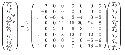
To this end, I used the EDF generators corresponding to the central and tensor parts of the nuclear Skyrme interaction [33,34,35,31,36], which is composed of eight terms ($m$=8), that is,

$$\left(\!\!\begin{array}{l} \hat{V}^\rho_0 \\ \hat{V}^\rho_1 \\ \h... ...T}_2 \\ \hat{T}_2^\sigma \\ \hat{T}_e \\ \hat{T}_o \\ \end{array}\!\!\!\right),$$ (5)

where $\hat{T}_0=\hat{\delta}$, $\hat{T}_1=\tfrac{1}{2}(\bm{k}'^*{}^2+ \bm{k}^2)\hat{\delta}$, $\hat{T}_2=(\bm{k}'^*\cdot\bm{k})\hat{\delta}$, and $\hat{\delta}$ is a two-body local zero-range potential, $\hat{\delta}=\delta(\bm{r}_1-\bm{r}_2)\delta(\bm{r}_1-\bm{r}'_1)\delta(\bm{r}_2-\bm{r}'_2)$. The standard relative-momentum operators are defined as $\bm{k}=(\bm{\nabla}_1-\bm{\nabla}_2)/2i$ and $\bm{k}'=(\bm{\nabla}'_1-\bm{\nabla}'_2)/2i$, $\hat{T}_i^\sigma=\hat{T}_i\hat{P}_{\sigma}$ for $\hat{P}_{\sigma}=\tfrac{1}{2}(1+\bm{\sigma}_1\cdot\bm{\sigma}_2)$, and $\hat{T}_e =\tfrac{1}{2} ({\bm{k}}^{\prime *}\cdot\hat{{\mathsf S}}\cdot{\bm{k}}^{\prime *} + \bm{k} \cdot\hat{{\mathsf S}}\cdot\bm{k})$ and $\hat{T}_o ={\bm{k}}^{\prime *}\cdot\hat{{\mathsf S}} \cdot\bm{k}$ for $\hat{{\mathsf S}}^{ab} =\tfrac{3}{2}\big(\sigma_1^a \sigma_2^b +\sigma_1^b \sigma_2^a\big) - \delta_{ab}\bm{\sigma}_1\cdot \bm{\sigma}_2$.

Numerical coefficients appearing in Eq. (5) were chosen in such a way that each of the eight EDF generators gives (in spherical nuclei) one specific term of the EDF [37,38,36], namely,

$$\begin{array}{rclcrcl} {V}^\rho_t\left[\rho\right]&=&\rho_t(\... ...{\mathsf J}_t(\bm{r})\cdot{\mathsf J}_t(\bm{r}), \\ \end{array}$$ (6)

where index $t$ refers to the isoscalar ($t$=0) or isovector ($t$=1) densities, $\Delta\rho_t(\bm{r})$ stands for the Laplacian of the density, and ${\tau}_t(\bm{r})=\big[(\bm{\nabla}\cdot\bm{\nabla}') {\rho}_t(\bm{r},\bm{r}')\big]_{\bm{r}=\bm{r}'}$ and ${{\mathsf J}}^{ab}_t(\bm{r})=\tfrac{1}{2i}\big[ (\nabla_a - \nabla_a') s^b_t(\bm{r},\bm{r}')\big]_{\bm{r}=\bm{r}'}$ are the standard quasilocal kinetic and spin-current densities, respectively.

For the proof-of-principle application presented in this work, instead of the average value of the true many-body Hamiltonian, I used the Gogny EDF [39] in the D1S parametrization [40], that is, $\langle\Psi\vert\hat{H}\vert\Psi\rangle\rightarrow{}E_{\text{Gogny}}\left[\rho\right]$. In this way, I aimed at obtaining a Gogny-equivalent quasilocal Skyrme EDF. That both types of EDFs can be linked to one another is already known from findings of Refs. [41,42], where this fact was demonstrated within the DME and effective theory; here I aim at testing this equivalence in terms of the ab initio-like methodology proposed in this work. Since both functionals contain terms generated by the zero-range spin-orbit and density-dependent operators, these were left untouched, and in the left-hand side of Eq. (4) only the part of the Gogny EDF generated by the finite-range potentials was used.

Numerical results presented below were obtained using the code HFODD (v2.75c) [43], which is the only existing code capable of treating the Gogny and Skyrme functionals simultaneously and within the same numerical infrastructure, see the Supplemental Material [44] for details. Calculations were performed for eight doubly magic nuclei, $^{16}$O, $^{40,48}$Ca, $^{56,78}$Ni, $^{100,132}$Sn, and $^{208}$Pb. For each nucleus, I used either of the eight Lagrange multipliers, ${\lambda }_t^\rho$, ${\lambda }_t^{\Delta \rho }$, ${\lambda }_t^\tau$, or ${\lambda }_t^J$ (for $t$=0,1) equal to one of the 21 integer values between $-$10 and +10MeVfm$^n$, where $n$=3 for ${\lambda }_t^\rho$ and $n$=5 for the other ones. Altogether, this gave me 1344 values of the Gogny energies $E(\lambda^j)$, to which the eight coupling constants of the Skyrme EDF, $C_t^\rho$, $C_t^{\Delta\rho}$, $C_t^\tau$, and $C_t^J$ (for $t$=0,1) were adjusted in Eq. (4).

Table 1: The Skyrme EDF S1Sd and S1Se coupling constants obtained in this work as the ab initio-equivalent Gogny EDF D1S [40].

		S1Sd			S1Se
		$t=0$	$t=1$		$t=0$	$t=1$
$C^\rho_t$	(MeVfm$^3$)	$-$603.82(22)	$$484(4)		$-$605.41(16)	$$509(3)
$C^{\Delta\rho}_t$	(MeVfm$^5$)	$-$73.25(14)	$$48(3)		$-$74.82(12)	$$41(2)
$C^\tau_t$	(MeVfm$^5$)	$$77.95(23)	$-$78(3)		$$79.73(16)	$-$98(2)
$C^J_t$	(MeVfm$^5$)	$$24.9(1.2)	$$71(3)		$$ 0	$$ 0

Figure 1: (Color online) Gogny energies [lines, left-hand side of Eq. (4)] compared with the EDF estimates [symbols, right-hand side of Eq. (4)] obtained for the Skyrme EDF S1Sd coupling constants given in Table 1. Calculations were performed in $^{208}$Pb in function of the eight Lagrange multipliers ${\lambda }_t^\rho$, ${\lambda }_t^{\Delta \rho }$, ${\lambda }_t^\tau$, and ${\lambda }_t^J$ for $t$=0,1. The inset shows residuals of the adjustment in per cent.

The coupling constants S1Sd obtained by such an adjustment are shown in Table 1. Their standard uncertainties were obtained within the standard regression analysis presented, e.g., in Refs. [45,46]. The adjusted coupling constants reproduced the Gogny energies in Eq. (4) with a very high accuracy: the relative rms deviation between left- and right-hand sides of Eq. (4) is only 0.014%. This is also illustrated in Fig. 1, where differences between symbols and lines cannot be seen at all, while the inset shows that the relative residuals of the adjustment do not exceed 0.050%. Analogous plots for other nuclei are collected in the Supplemental Material [44].

Table 2: Gogny EDF D1S ground-state energies $E_G$ (b) of eight doubly magic nuclei (a) compared to energies $E$ (c) calculated using the Skyrme EDF S1Sd, Table 1, and shown together with their propagated uncertainties $\Delta {E}$. Column (d) shows the residuals $\delta {E}=E-E_G$ and columns (e) and (f) give ratios of residuals with respect to energies $E$ and propagated uncertainties $\Delta {E}$, respectively. All energies are in MeV.

	$E_G$		$E$	$\delta{E}$	$\delta{E}/\vert E\vert$	$\delta{E}/\Delta{E}$
(a)	(b)		(c)	(d)	(e)	(f)
$^{16}$O	$-$129.626		$-$129.56(4)	$$0.07	$$0.05%	$$ 2
$^{ 40}$Ca	$-$344.663		$-$346.01(6)	$-$1.35	$-$0.39%	$-$23
$^{ 48}$Ca	$-$416.829		$-$418.10(6)	$-$1.27	$-$0.30%	$-$20
$^{ 56}$Ni	$-$483.820		$-$485.31(6)	$-$1.49	$-$0.31%	$-$27
$^{ 78}$Ni	$-$640.598		$-$642.37(6)	$-$1.78	$-$0.28%	$-$28
$^{100}$Sn	$-$830.896		$-$833.19(6)	$-$2.29	$-$0.28%	$-$39
$^{132}$Sn	$-$1103.246		$-$1106.51(8)	$-$3.26	$-$0.30%	$-$42
$^{208}$Pb	$-$1638.330		$-$1640.96(8)	$-$2.63	$-$0.16%	$-$32
rms	n.a.		n.a.	$$1.99	$$0.28%	$$29

Table 2 compares the ground-state energies $E_G$ calculated using the original Gogny EDF D1S with energies $E$ obtained by the minimization of the Gogny-equivalent Skyrme EDF S1Sd. Propagated uncertainties $\Delta {E}$ of $E$ were calculated using the covariance matrix related to the adjustment of coupling constants [45,46], see the Supplemental Material [44]. We see that the Skyrme EDF S1Sd again reproduces the Gogny-EDF results with a very high accuracy: the relative rms deviations between these two functionals is only 0.28%. This is much better than the accuracy obtained within the DME [47], see the comparison presented in the Supplemental Material [44]. One can conclude that the simple eight-dimensional Gogny-equivalent Skyrme EDF with ab initio-derived coupling constants of Eq. (2) very well describes the full Gogny energies. We note here that the coupling constants were adjusted only to energies. In the Supplemental Material [44], I also show the analogous very good agreement obtained for the proton rms radii. This points to a well-built EDF, which along with the total energies properly describes one-body observables.

On the absolute scale, the corresponding rms deviation of energies is 1.99MeV, which is 29 times higher than the rms average of the propagated uncertainties, see Table 2. It means that the differences between the Gogny results and Gogny-equivalent Skyrme-EDF results are still significantly larger than the uncertainties of the adjustment, which gives a clear signal for missing terms in the eight-dimensional model EDF of Eq. (4).

The method also allows for testing the impact of removing terms from the model EDF. For example, setting the two spin-current coupling constants to zero, $C_0^J=C_1^J=0$, one obtains a six-dimensional model that gives another Gogny-equivalent Skyrme EDF S1Se, with coupling constants shown in Tables 1. Such model is only marginally worse, with the absolute and relative rms deviations of energies now increased to 2.34MeV and 0.40%, respectively, see the Supplemental Material [44] for detailed results.

In conclusion, I proposed a novel method of obtaining ab initio-equivalent model EDFs. The main idea is in replacing the standard-DFT use of an external one-body potential by the use of two-body, three-body, etc., EDF generators. This probes the reaction of the system with respect to the same operators that are used to construct the model EDFs. The new method amounts to performing ab initio calculations with simple constraints on a finite set of well-defined operators added to the many-body Hamiltonian, and thus is perfectly manageable.

The method is also able to give us a quantitative information on whether a given model EDF is adequate for the proper description of the physical system being studied. Indeed, if the adjustment of the coupling constants fails to be accurate enough, we obtain a clear signal that the set of proposed EDF generators is inadequate. Then, another or extended model EDF should be tried. In this way, through ab initio derivations in nuclei, one may be able to evaluate relative merits of using the zero-range higher-order [48], finite-range regularized [49], three-body or four-body [50], or gradient-dependent three-body [51] pseudopotentials, which are currently being developed and implemented in nuclear EDF approaches.

It is very important that the proposed method is based on studying specific finite systems and does not rely on assumptions valid only in infinite or semi-infinite systems. The proposed ab initio derivations can be performed in few systems, for which the ab initio calculations are possible, e.g., in light closed-shell nuclei, and then the derived EDFs can be applied to more complicated, open-shell or heavy nuclei, so as to test the overall predictive power of the method. It is also essential that the ab initio-equivalent EDFs are specific to particular physical systems, and when applied to systems at different energies or densities will yield parametrically energy- or density-dependent running coupling constants. Needless to say that the proposed method can easily be extended to deriving time-odd or pairing terms of the EDFs. Another fascinating extension would be to use the same method not only to match energies, like in Eq. (4), but also ab initio-derived kernels [52,53].

Very interesting discussions with Witek Nazarewicz are gratefully acknowledged. This work was supported in part by the Academy of Finland and University of Jyväskylä within the FIDIPRO program, by the Polish National Science Center under Contract No. 2012/07/B/ST2/03907, and by the ERANET-NuPNET grant SARFEN of the Polish National Centre for Research and Development (NCBiR). We acknowledge the CSC-IT Center for Science Ltd., Finland, for the allocation of computational resources.