Divergence in the Abnormal Density

In the DFT-HFB approach, the starting point is the Energy Density Functional (EDF) $\mathcal{H}[\rho,\tilde\rho]$, where $\rho$ is the particle density and $\tilde\rho$ is the abnormal density:

$$\rho(\mathbf{r_2}\sigma_2\tau_2,\mathbf{r_1}\sigma_1\tau_1) =\!\! \langle\Phi\vert a^{\dagger}_{\mathbf{r_1}\sigma_1\tau_1}a_{\mathbf{r_2}\sigma_2\tau_2}\vert\Phi\rangle,$$ (16)

$$\tilde\rho(\mathbf{r_2}\sigma_2\tau_2,\mathbf{r_1}\sigma_1\tau_1) =\!\! -2\sigma_1\langle\Phi\vert a_{\mathbf{r_1}-\sigma_1\tau_1}a_{\mathbf{r_2}\sigma_2\tau_2}\vert\Phi\rangle,$$ (17)

where $a$ and $a^{\dagger}$ are the particle annihilation and creation operators, respectively, and $\vert\Phi\rangle$ is the HFB state. In the following, we assume that $\vert\Phi\rangle$ is a product of the neutron and proton states, $\vert\Phi_{\nu}\rangle\vert\Phi_{\pi}\rangle$. Therefore, the neutron and proton wave functions are not coupled, and in the notation below we can, for simplicity, omit the isospin index with the understanding that all equations are separately valid for neutrons and protons.

For the HFB state $\vert\Phi\rangle$, the particle and abnormal densities can be written as [12]:

$$\rho(\mathbf{r_2}\sigma_2,\mathbf{r_1}\sigma_1) = \sum_{E_i>0}\varphi_{2i}(\mathbf{r_2}\sigma_2)\varphi_{2i}^*(\mathbf{r_1}\sigma_1),$$ (18)

$$\tilde\rho(\mathbf{r_2}\sigma_2,\mathbf{r_1}\sigma_1) = -\sum_{E_i>0}\varphi_{2i}(\mathbf{r_2}\sigma_2)\varphi_{1i}^*(\mathbf{r_1}\sigma_1),$$ (19)

where the two-component quasiparticle wave function $\varphi$ is the solution of the HFB equation:

$$\sum_{\sigma_1}\int d^3\mathbf{r_1}\left[\begin{array}{cc}h_{\mu}... ..._1)&-h_{\mu}(\mathbf{r_2}\sigma_2,\mathbf{r_1}\sigma_1)\end{array}\right]\times$$

$$\times\left[\begin{array}{c}\varphi_{1i}(\mathbf{r_1}\sigma_1)\\ ... ...(\mathbf{r_2}\sigma_2)\\ \varphi_{2i}(\mathbf{r_2}\sigma_2)\end{array}\right],$$ (20)

for a given quasiparticle energy $E_i$.

The HFB equations are a result of variational minimization of the energy density functional $\mathcal{H}[\rho,\tilde\rho]$ with the constraint of the mean value of particles kept constant:

$$\left.\delta\mathcal{H}\right\vert _{\langle \hat N\rangle=N}=0.$$ (21)

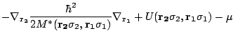
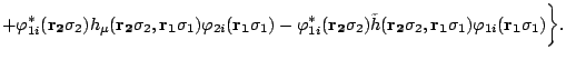
This condition defines the s.p. Hamiltonian $h_{\mu}$ and the pairing Hamiltonian $\tilde h$ in the HFB equations (20):

$${h_{\mu}(\mathbf{r_2}\sigma_2,\mathbf{r_1}\sigma_1)=\frac{\delta\... ...}[\rho,\tilde\rho]}{\delta\rho(\mathbf{r_1}\sigma_1,\mathbf{r_2}\sigma_2)}-\mu}$$

$$= -{\mathbf{\nabla}_{\mathbf{r_2}}}\frac{\hbar^2}{2M^*(\mathbf{r_2}... ...athbf{\nabla}_{\mathbf{r_1}}} +U(\mathbf{r_2}\sigma_2,\mathbf{r_1}\sigma_1)-\mu$$

$${\tilde h(\mathbf{r_2}\sigma_2,\mathbf{r_1}\sigma_1)=\frac{\delta... ...rho,\tilde\rho]}{\delta\tilde\rho(\mathbf{r_1}\sigma_2,\mathbf{r_2}\sigma_2)}},$$

where $M^*$ is the effective mass and $U$ is the self-consistent mean-field potential. In the following derivations, the spin-orbit term is omitted as unimportant in the regularization scheme, although it is, of course, always included in calculations.

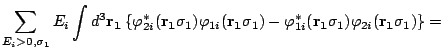
By multiplying the HFB equations (20) by vector $[\varphi_{2i}^*,-\varphi_{1i}^*]$, integrating over coordinates and summing over all the positive energy HFB solutions, one obtains:

$${\sum_{E_i>0,\sigma_2} E_i\int d^3\mathbf{r_2} \left[\begin{array... ...mathbf{r_2}\sigma_2)\\ \varphi_{2i}(\mathbf{r_2}\sigma_2) \end{array}\right]=}$$

$$=\sum_{E_i>0,\sigma_1\sigma_2} \int d^3\mathbf{r_1}d^3\mathbf{r_2... ...(\mathbf{r_1}\sigma_1)\\ \varphi_{2i}(\mathbf{r_1}\sigma_1) \end{array}\right]$$ (24)

i.e.,

$${\sum_{E_i>0,\sigma_1} E_i \int d^3\mathbf{r_1} \left\{\varphi_{2... ...varphi_{1i}^*(\mathbf{r_1}\sigma_1)\varphi_{2i}(\mathbf{r_1}\sigma_1)\right\}=}$$

$$=\sum_{E_i>0,\sigma_1\sigma_2} \int d^3\mathbf{r_1}d^3\mathbf{r_2... ...h(\mathbf{r_2}\sigma_2,\mathbf{r_1}\sigma_1)\varphi_{2i}(\mathbf{r_1}\sigma_1)+$$

$$+\varphi_{1i}^*(\mathbf{r_2}\sigma_2)h_{\mu}(\mathbf{r_2}\sigma_2... ...bf{r_2}\sigma_2,\mathbf{r_1}\sigma_1)\varphi_{1i}(\mathbf{r_1}\sigma_1)\bigg\}.$$ (25)

Since for every HFB solution $([\varphi_{1i},\varphi_{2i}],E_i)$ there exists also an orthogonal solution $([\varphi_{2i},-\varphi_{1i}],-E_i)$, the left-hand side of Eq. (25) vanishes as a sum over scalar products of orthogonal wave functions.

For local and spin-independent Hamiltonians $h_{\mu}$ and $\tilde h$, Eqs. (23) and (23) read

$$h_{\mu}(\mathbf{r_2}\sigma_2,\mathbf{r_1}\sigma_1) = -\mathbf{\nabla}_{\mathbf{r_2}}\frac{\hbar^2}{2M^*(\mathbf{r_2})}... ...(\mathbf{r_2})-\mu)\delta(\mathbf{r_2}-\mathbf{r_1})\delta_{\sigma_2,\sigma_1},$$ (26)

$$\tilde h(\mathbf{r_2}\sigma_2,\mathbf{r_1}\sigma_1) = \tilde h(\mathbf{r_2})\delta(\mathbf{r_2}-\mathbf{r_1})\delta_{\sigma_2,\sigma_1}.$$ (27)

Note that for an attractive pairing force, the local pairing potential $\tilde h(\mathbf{r})=-\Delta(\mathbf{r})$ is negative, where $\Delta(\mathbf{r})$ is the standard position-dependent pairing gap. By defining function $\mathcal F_{\epsilon_{\mbox{\rm\scriptsize {cut}}}}$ as

$$\sum_{E_i>0,\sigma} \left[\varphi_{1i}(\mathbf{r_2}\sigma)\va... ...lon_{\mbox{\rm\scriptsize {cut}}}}(\mathbf{r_2}-\mathbf{r_1}).$$ (28)

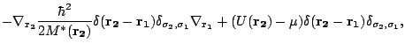
and using expression (19) for the abnormal density, one obtains after integrating the kinetic-energy term by parts:

$$0 = -\int d^3\mathbf{r_1}d^3\mathbf{r_2}\delta(\mathbf{r_2}-\mathbf{r... ...r_1}} +U(\mathbf{r_2})-\mu\right)2\tilde\rho(\mathbf{r_1},\mathbf{r_2})\right]=$$

$$= -\int d^3\mathbf{r}d^3\mathbf{x}\delta(\mathbf{x})\left[\tilde h(... ...-\mu\right)2\tilde\rho(\mathbf{r}-\mathbf{x}/2,\mathbf{r}+\mathbf{x}/2)\right],$$ (29)

where

$$\mathbf{r} = \frac{\mathbf{r_1}+\mathbf{r_2}}{2},$$ (30)

$$\mathbf{x} = \mathbf{r_2}-\mathbf{r_1},$$ (31)

and

$$\rho(\mathbf{r_2},\mathbf{r_1}) = \sum_{\sigma}\rho(\mathbf{r_2}\sigma,\mathbf{r_1}\sigma),$$ (32)

$$\tilde\rho(\mathbf{r_2},\mathbf{r_1}) = \sum_{\sigma}\tilde\rho(\mathbf{r_2}\sigma,\mathbf{r_1}\sigma).$$ (33)

When the summation over positive quasiparticle energies is extended to infinity, the completeness relation implies that

$$\mathcal F_{\epsilon_{\mbox{\rm\scriptsize {cut}}}}(\mathbf{r_2}-\mathbf{r_1})=\delta(\mathbf{r_2}-\mathbf{r_1}),$$ (34)

and the only term in Eq. (29) capable of canceling out this singularity is $\nabla_{\mathbf{x}}^2\tilde\rho(\mathbf{r}-\mathbf{x}/2,\mathbf{r}+\mathbf{x}/2)$. Therefore, the Laplacian of the abnormal density $\nabla_{\mathbf{x}}^2\tilde\rho(\mathbf{r}-\mathbf{x}/2,\mathbf{r}+\mathbf{x}/2)$ must be singular at $\mathbf{x}=0$. Moreover, using the expression

$$\nabla^2\frac{1}{\vert\mathbf{r}\vert}=-4\pi\delta(\mathbf{r}),$$ (35)

it is clear that due to the zero-range pairing interaction abnormal density $\tilde\rho$ has an ultraviolet $1/x$ divergence:

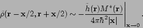$$\left.\tilde\rho(\mathbf{r}-\mathbf{x}/2,\mathbf{r}+\mathbf{x... ...^2\vert\mathbf{x}\vert}\right\vert _{\mathbf{x}\rightarrow 0}.$$ (36)