The classical model of chiral rotation was briefly introduced in Ref. [32];
here we give its more detailed description and discussion.
In order to define the model, we
begin with elementary considerations related to the dynamics of rigid
bodies. By a classical gyroscope we understand an axial-shape rigid
body with moments of inertia,
![]() and
and
![]() ,
with respect to the symmetry axis and an axis perpendicular to it,
respectively. Such a body spins with fixed angular frequency
,
with respect to the symmetry axis and an axis perpendicular to it,
respectively. Such a body spins with fixed angular frequency ![]() around its symmetry axis; one can imagine that this motion is ensured
by a motor and frequency regulator such that
around its symmetry axis; one can imagine that this motion is ensured
by a motor and frequency regulator such that ![]() is strictly
constant in time.
is strictly
constant in time.
Furthermore, let us imagine that the spinning body is
rigidly mounted on another rigid body that has triaxial inertia tensor and
three moments of inertia
![]() ,
,
![]() , and
, and
![]() , with
respect to its short, medium, and long axis, respectively. Then, the
angular frequency
, with
respect to its short, medium, and long axis, respectively. Then, the
angular frequency ![]() is maintained fixed with respect to the
triaxial body, irrespective of how the whole device moves, and the
angular frequency vector
is maintained fixed with respect to the
triaxial body, irrespective of how the whole device moves, and the
angular frequency vector
![]() has by definition three
time-independent components
has by definition three
time-independent components ![]() ,
, ![]() , and
, and ![]() .
To simplify our considerations let us assume that the
axis of the gyroscope coincides with the short axis of the triaxial
body, i.e.,
.
To simplify our considerations let us assume that the
axis of the gyroscope coincides with the short axis of the triaxial
body, i.e., ![]() =
=![]() ,
, ![]() =0, and
=0, and ![]() =0.
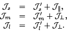
In this case the principal axes of the tensor of inertia of the whole device
coincide with those of the triaxial body, and the three moments of inertia of
the device read,
=0.
In this case the principal axes of the tensor of inertia of the whole device
coincide with those of the triaxial body, and the three moments of inertia of
the device read,
 |
(7) |
We assume that the device rotates with the total angular frequency
vector
![]() , which in the moving frame of the triaxial body
has components
, which in the moving frame of the triaxial body
has components ![]() ,
, ![]() , and
, and ![]() . In general,
these components may vary with time, although later we study only
such a motion of the device when they are time-independent. The kinetic
energy of the device is the sum of that of the triaxial body and gyroscope,
. In general,
these components may vary with time, although later we study only
such a motion of the device when they are time-independent. The kinetic
energy of the device is the sum of that of the triaxial body and gyroscope,
| (8) |
| (9) | |||
| (10) |
It is obvious that if we add two other gyroscopes aligned
with the medium and long axes and spinning with spins ![]() and
and
![]() , respectively, the second term can be simply written as a
scalar product
, respectively, the second term can be simply written as a
scalar product
![]() , where vector
, where vector ![]() has
components
has
components ![]() ,
, ![]() , and
, and ![]() . In this case, the total moment of
inertia
. In this case, the total moment of
inertia
![]() will be a sum of contributions from the triaxial body
and three gyroscopes. We note in passing that exactly the same
result is obtained for a single spherical gyroscope,
will be a sum of contributions from the triaxial body
and three gyroscopes. We note in passing that exactly the same
result is obtained for a single spherical gyroscope,
![]() , tilted with respect to the principal
axes of the triaxial body in such a way that it has spin components
equal to
, tilted with respect to the principal
axes of the triaxial body in such a way that it has spin components
equal to ![]() ,
, ![]() , and
, and ![]() .
.
The total angular momentum,
![]() , of the system reads
, of the system reads
Equations of motion for the model can be derived in the following
way. As for any vector, the time derivatives of the angular momentum vector,
![]() - taken in the
laboratory frame and
- taken in the
laboratory frame and
![]() - taken
in a frame rotating with angular frequency
- taken
in a frame rotating with angular frequency
![]() , are related by the formula
, are related by the formula
![]() [43]. Since the angular momentum is
conserved in the laboratory frame,
[43]. Since the angular momentum is
conserved in the laboratory frame,
![]() ,
one obtains the Euler equations [43] for the time
evolution of the angular-momentum vector in the body-fixed frame,
,
one obtains the Euler equations [43] for the time
evolution of the angular-momentum vector in the body-fixed frame,
The mean-field cranking approximation can only account for the
so-called uniform rotations, in which the mean angular-momentum
vector is constant in the intrinsic frame of the nucleus,
![]() . Because of that, we restrict the
classical model studied here to such uniform rotations.
Due to Eq. (12), for uniform rotations also the
angular frequency vector is constant in the intrinsic frame.
The Euler equations (16) now take the form
. Because of that, we restrict the
classical model studied here to such uniform rotations.
Due to Eq. (12), for uniform rotations also the
angular frequency vector is constant in the intrinsic frame.
The Euler equations (16) now take the form
![]() , and require that
, and require that
![]() and
and
![]() be parallel. The same condition holds for the HF solutions
and is known as the Kerman-Onishi theorem; see Section 2
and [37]. The Euler equations can now be easily solved for the
considered classical model. However, to show further analogies with
the HF method, in what follows we find the uniform solutions by
employing a variational principle.
be parallel. The same condition holds for the HF solutions
and is known as the Kerman-Onishi theorem; see Section 2
and [37]. The Euler equations can now be easily solved for the
considered classical model. However, to show further analogies with
the HF method, in what follows we find the uniform solutions by
employing a variational principle.
According to the Hamilton's principle, motion of a mechanical system
can be found by making the action integral, ![]() , stationary.
The real uniform rotations obviously belong to a wider class of trial
motions with
, stationary.
The real uniform rotations obviously belong to a wider class of trial
motions with ![]() and
and
![]() being constant in the intrinsic frame,
but not necessarily parallel to one another. Within
this class, Lagrangian (13) does not depend on time.
Therefore, extremizing the action for a given value of
being constant in the intrinsic frame,
but not necessarily parallel to one another. Within
this class, Lagrangian (13) does not depend on time.
Therefore, extremizing the action for a given value of ![]() =
=
![]() reduces to
finding extrema of the Lagrangian as a function of the
intrinsic-frame components of
reduces to
finding extrema of the Lagrangian as a function of the
intrinsic-frame components of
![]() . Since
. Since ![]() , the
Routhian (15) can be equally well used for this
purpose. This provides us with a bridge between the classical model and the
quantum cranking theory, where an analogous Routhian
(1) is minimized in the space of the trial
wave-functions.
, the
Routhian (15) can be equally well used for this
purpose. This provides us with a bridge between the classical model and the
quantum cranking theory, where an analogous Routhian
(1) is minimized in the space of the trial
wave-functions.
Extrema of ![]() with respect to the intrinsic-frame components of
with respect to the intrinsic-frame components of
![]() at a given length of
at a given length of ![]() can be found by using a
Lagrange multiplier,
can be found by using a
Lagrange multiplier,
![]() , for
, for
![]() (the factor
(the factor
![]() being added for later convenience). We continue further
derivations for the case of two gyroscopes aligned along the
being added for later convenience). We continue further
derivations for the case of two gyroscopes aligned along the ![]() and
and
![]() axes, as dictated by the microscopic results presented in Section 3.4, i.e., we employ the classical model for
axes, as dictated by the microscopic results presented in Section 3.4, i.e., we employ the classical model for ![]() =0.
Setting to zero the
derivatives of the quantity
=0.
Setting to zero the
derivatives of the quantity
| (17) |
|
If
![]() then both
then both
![]() and
and ![]() lie in the
lie in the
![]() -
-![]() plane. This gives planar solutions, for which the chiral
symmetry is not broken. All values of
plane. This gives planar solutions, for which the chiral
symmetry is not broken. All values of ![]() are allowed, and the
Lagrange multiplier must be determined from the length of
are allowed, and the
Lagrange multiplier must be determined from the length of
![]() calculated in the obvious way from (18) and
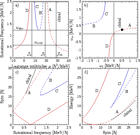
(20). Figure 5a shows
calculated in the obvious way from (18) and
(20). Figure 5a shows ![]() versus
versus ![]() for sample model parameters, extracted from the
for sample model parameters, extracted from the ![]() La HF PAC solutions with
the SLy4 force with no time-odd fields, and listed in
Table 1. The solutions marked as A and D exist for all
values of
La HF PAC solutions with
the SLy4 force with no time-odd fields, and listed in
Table 1. The solutions marked as A and D exist for all
values of ![]() , while above some threshold frequency,
, while above some threshold frequency,
![]() , two more solutions appear, B and C. This threshold
frequency can be determined by finding the minimum of
, two more solutions appear, B and C. This threshold
frequency can be determined by finding the minimum of ![]() in
function of
in
function of ![]() , and reads
, and reads
 |
(21) |
For ![]() =
=
![]() , all values of
, all values of ![]() are allowed, while
components in the
are allowed, while
components in the ![]() -
-![]() plane are fixed at
plane are fixed at
![]() and
and
![]() .
Consequently, the angular momentum has non-zero components along all
three axes, and the chiral symmetry is broken. For each value of
.
Consequently, the angular momentum has non-zero components along all
three axes, and the chiral symmetry is broken. For each value of
![]() , there are two cases differing by the sign of
, there are two cases differing by the sign of
![]() ,
and thus giving the chiral doublet. The fact that
,
and thus giving the chiral doublet. The fact that
![]() and
and
![]() are constant leads to the principal conclusion that
chiral solutions cannot exist for
are constant leads to the principal conclusion that
chiral solutions cannot exist for ![]() smaller than the critical
frequency
smaller than the critical
frequency
In the
![]() space, the four planar solutions form a
hyperbola in the
space, the four planar solutions form a
hyperbola in the ![]() -
-![]() plane, while the chiral doublet corresponds
to a straight line perpendicular to that plane. These curves are
shown in Fig. 5b. Figure 5c gives the
angular momentum in function of rotational frequency for all the
presented bands. With increasing
plane, while the chiral doublet corresponds
to a straight line perpendicular to that plane. These curves are
shown in Fig. 5b. Figure 5c gives the
angular momentum in function of rotational frequency for all the
presented bands. With increasing ![]() , the so-called dynamical moment,
, the so-called dynamical moment,
![]() , asymptotically approaches
, asymptotically approaches
![]() for bands A and B, and
for bands A and B, and
![]() for bands C and D. For the
chiral band,
for bands C and D. For the
chiral band, ![]() is exactly proportional to
is exactly proportional to ![]() with the
coefficient
with the
coefficient
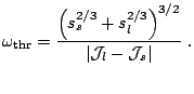
![]() . Thus, the critical spin,
. Thus, the critical spin,
![]() ,
corresponding to the critical frequency (22) reads
,
corresponding to the critical frequency (22) reads
Figure 5d summarizes the energies in function of spin.
The spin quantum number, ![]() , is related to the length,
, is related to the length, ![]() , of the
angular momentum vector,
, of the
angular momentum vector, ![]() , by the condition
, by the condition
![]() . At
low angular momenta, the yrast line coincides with the planar band D.
Then it continues along the planar solution A. Since the moment of
inertia
. At
low angular momenta, the yrast line coincides with the planar band D.
Then it continues along the planar solution A. Since the moment of
inertia
![]() is the largest, beyond the critical frequency the
chiral solution becomes yrast, thereby yielding good prospects for
experimental observation.
is the largest, beyond the critical frequency the
chiral solution becomes yrast, thereby yielding good prospects for
experimental observation.
Altogether, the classical model described here is defined by five
parameters,
![]() ,
,
![]() ,
,
![]() ,
, ![]() , and
, and ![]() , which
are extracted form the microscopic HF PAC calculations and listed
in Table 1. The model can then be applied to predict
properties of the planar and chiral TAC bands, and these predictions
can be compared with the HF TAC results. Such a comparison is
presented and discussed in the following Sections.
, which
are extracted form the microscopic HF PAC calculations and listed
in Table 1. The model can then be applied to predict
properties of the planar and chiral TAC bands, and these predictions
can be compared with the HF TAC results. Such a comparison is
presented and discussed in the following Sections.
![$\displaystyle \omega_{\text{crit}}^{\text{clas}}=\left[\left(\frac{s_s}{\mathca...
...right)^2 +\left(\frac{s_l}{\mathcal{J}_m-\mathcal{J}_l}\right)^2\right]^{1/2}~.$](img223.png)