The survey of ISB corrections in $10\leq A \leq 74$ nuclei

Table 2: Results of calculations for the superallowed transitions measured experimentally. Shown are: the empirical $ft$-values [5]; SV values of $\delta_{\rm C}$ calculated by projecting from the $\vert\varphi_{\rm X}\rangle,\vert\varphi_{\rm Y}\rangle$, and $\vert\varphi_{\rm Z}\rangle$ Slater determinants, see Sec. 3.1; recommended mean $\delta_{\rm C}^{{\rm (SV)}}$ corrections (see Sec. 3.3) and the corresponding ${\cal F}t$-values; empirical $\delta_{\rm C}^{{\rm (exp)}}$ corrections calculated by using Eq. (23); contributions coming from the individual transitions to the $\chi^2$ budget in the confidence-level test; mean $\delta_{\rm C}^{{\rm (SHZ2)}}$ corrections and the corresponding ${\cal F}t$-values.

Parent	$ft$	$\quad$	$\delta_{\rm C}^{\rm (X)}$	$\delta_{\rm C}^{\rm (Y)}$	$\delta_{\rm C}^{\rm (Z)}$	$\quad$	$\delta_{\rm C}^{{\rm (SV)}}~\strut$	${\cal F}t~~~~~\strut$	$\quad$	$\delta_{\rm C}^{{\rm (exp)}}~\strut$	$\chi^2_i$	$\quad$	$\delta_{\rm C}^{{\rm (SHZ2)}}~~\strut$	${\cal F}t~~~~~\strut$
nucleus	(s)		(%)	(%)	(%)		(%)	(s)		(%)			(%)	(s)
$T_z=-1:$
$^{10}$C	3041.7(43)		0.559	0.559	0.823		0.65(14)	3062.1(62)		0.37(15)	3.7		0.462(65)	3067.8(49)
$^{14}$O	3042.3(11)		0.303	0.303	0.303		0.303(30)	3072.3(21)		0.36(06)	0.8		0.480(48)	3066.9(24)
$^{22}$Mg	3052.0(70)		0.243	0.243	0.417		0.301(87)	3080.5(75)		0.62(23)	1.9		0.342(49)	3079.2(72)
$^{34}$Ar	3052.7(82)		0.865	0.997	1.475		1.11(29)	3056(12)		0.63(27)	3.1		1.08(42)	3057(15)
$T_z=0:$
$^{26}$Al	3036.9(09)		0.308	0.308	0.494		0.370(95)	3070.5(31)		0.37(04)	0.0		0.307(62)	3072.5(23)
$^{34}$Cl	3049.4(11)		0.809	0.679	1.504		1.00(38)	3060(12)		0.65(05)	48.4		0.83(50)	3065(15)
$^{42}$Sc	3047.6(12)		--	--	--		0.77(27)	3069.2(85)		0.72(06)	0.5		0.70(32)	3071(10)
$^{46}$V	3049.5(08)		0.486	0.486	0.759		0.58(14)	3074.6(47)		0.71(06)	4.5		0.375(96)	3080.9(35)
$^{50}$Mn	3048.4(07)		0.460	0.460	0.740		0.55(14)	3074.1(47)		0.67(07)	3.1		0.39(13)	3079.2(45)
$^{54}$Co	3050.8(10)		0.622	0.622	0.671		0.638(68)	3074.0(32)		0.75(08)	2.0		0.51(20)	3078.0(66)
$^{62}$Ga	3074.1(11)		0.925	0.840	0.881		0.882(95)	3090.0(42)		1.51(09)	44.0		0.49(11)	3102.3(45)
$^{74}$Rb	3084.9(77)		2.054	1.995	1.273		1.77(40)	3073(15)		1.86(27)	0.1		0.90(22)	3101(11)
							$\overline{{\cal F}t}=$	3073.6(12)		$\chi^2 =$	112.2		$\overline{{\cal F}t}=$	3075.0(12)
							$\vert V_{\rm ud}\vert=$	0.97397(27)		$\chi_d^2 =$	10.2		$\vert V_{\rm ud}\vert=$	0.97374(27)
								0.99935(67)						0.99890(67)

Table 3: Similar as in Table 2, except for the unmeasured transitions.

Parent	$\delta_{\rm C}^{\rm (X)}$	$\delta_{\rm C}^{\rm (Y)}$	$\delta_{\rm C}^{\rm (Z)}$	$\quad$	$\delta_{\rm C}^{\rm (SV)}$	$\quad$	$\delta_{\rm C}^{\rm (SHZ2)}$
nucleus	(%)	(%)	(%)		(%)		(%)
$T_z=-1:$
$^{18}$Ne	2.031	1.064	1.142		1.41(46)		0.72(30)
$^{26}$Si	0.399	0.399	0.597		0.47(10)		0.529(77)
$^{30}$S	1.731	1.260	1.272		1.42(26)		0.98(21)
$T_z=0:$
$^{18}$F	1.819	0.956	0.987		1.25(42)		0.42(24)
$^{22}$Na	0.255	0.255	0.535		0.35(14)		0.216(86)
$^{30}$P	1.506	0.974	1.009		1.16(27)		0.60(20)
$^{66}$As	0.956	0.925	1.694		1.19(38)		0.64(12)
$^{70}$Br	1.654	1.479	1.429		1.52(18)		1.10(52)

The results of our calculations are collected in Tables 2 and 3, and in Fig. 6. In addition, Fig. 7 shows the differences, $\delta_{\rm C}^{({\rm SV})}- \delta_{\rm C}^{({\rm HT})}$, between our results and those of Ref. [3]. In spite of clear differences between SV and HT, which can be seen for specific transitions including those for $A=10$, 34, and 62, both calculations reveal a similar increase of $\delta_{\rm C}$ versus $A$, at variance with the RPA calculations of Ref. [13], which also yield systematically smaller values.

Figure 6: (Color online) ISB corrections to the superallowed $0^+ \rightarrow 0^+$ $\beta$-decays calculated for (a) $T_z= -1 \rightarrow T_z =0$ and (b) $T_z= 0 \rightarrow T_z =1$ transitions. Our adopted values from Table 2 (circles with error bars) are compared with ISB corrections from Refs. [3] (dots, shaded band marks errors) and [13] (triangles).

Figure 7: Differences between the ISB corrections to the twelve accurately measured superallowed $0^+ \rightarrow 0^+$ $\beta$-transitions (excluding $A$=38) calculated in this work with SV and those of HT [3]. Circles and dots mark the $T_z= -1 \rightarrow T_z =0$ and $T_z= 0 \rightarrow T_z =1$ decays, respectively. The errors, calculated as $\sqrt{(\Delta \delta_{\rm C}^{\rm (SV)})^2 + (\Delta \delta_{\rm C}^{\rm (HT)})^2}$, are shown by shaded bands.

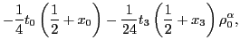
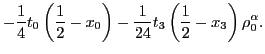
The ISB corrections used for further calculations of $V_{\rm ud}$ are collected in Table 2. Let us recall that our preference is to use the averaged corrections and that the $^{38}$K $\rightarrow$$^{38}$Ar transition has been disregarded. All other ingredients needed to compute the ${\cal F}t$-values, including radiative corrections $\delta_{\rm R}^\prime$ and $\delta_{\rm NS}$, are taken from Ref. [3], and the empirical $ft$-values are taken from Ref. [5]. For the sake of completeness, these empirical $ft$-values are also listed in Table 2.

Figure 8: The matrix element $\vert V_{\rm ud}\vert$ deduced from the superallowed $0^+ \rightarrow 0^+$ $\beta$-decay (dots) for different sets of the $\delta_{\rm C}$ corrections calculated in: (a) Ref. [3]; (b) Ref. [13] with NL3 and DD-ME2 Lagrangians; this work, using the averaged values of $\delta_{\rm C}$ with (c) SV and (d) SHZ2 functionals. Gray circles show ISB corrections with SV calculated at fixed shape-current orientations $X$, $Y$, and $Z$ (from left to right). Triangles mark values obtained from the pion-decay [39] and neutron-decay [10] studies. The open circle shows $\vert V_{\rm ud}\vert$ deduced from the $\beta$-decays in the $T=1/2$ mirror nuclei [40]

.

Figure 9: Similar as in Fig. 8 except for the unitarity condition (20).

In the error budget of the resulting ${\cal F}t$-values listed in Table 2, apart from errors in the $ft$ values and radiative corrections, we also included the uncertainties estimated for the calculated values of $\delta_{\rm C}$, see Sec. 3.3. To conform with HT, the average value $\overline{{\cal F}t} = 3073.6(12)$s was calculated by using the Gaussian-distribution-weighted formula. However, unlike HT, we do not apply any further corrections to $\overline{{\cal F}t}$. This leads to $\vert V_{\rm ud}\vert = 0.97397(27)$, which agrees very well with both the HT result [3], $\vert V_{\rm ud}^{{\rm (HT)}}\vert = 0.97418(26)$, and the central value obtained from the neutron decay $\vert V_{\rm ud}^{(\nu )}\vert = 0.9746(19)$ [10]. A survey of the $\vert V_{\rm ud}\vert$ values deduced by using different methods is given in Fig. 8. By combining the value of $\vert V_{\rm ud}\vert$ calculated here with those of $\vert V_{\rm us}\vert = 0.2252(9)$ and $\vert V_{\rm ub}\vert = 0.00389(44)$ of the 2010 Particle Data Group [10], one obtains

$$\vert V_{\rm ud}\vert^2 + \vert V_{\rm us}\vert^2 + \vert V_{\rm ub}\vert^2 = 0.99935(67),$$ (20)

which implies that the unitarity of the first row of the CKM matrix is satisfied with a precision better than 0.1%. A survey of the unitarity condition (20) is shown in Fig. 9.

It is worth noting that by using $\delta_{\rm C}$ values corresponding to the fixed current-shape orientations ( $\vert\varphi_{\rm X}\rangle$, $\vert\varphi_{\rm Y}\rangle$, or $\vert\varphi_{\rm Z}\rangle$) instead of their average, one still obtains compatible results for $\vert V_{\rm ud}\vert$ and unitarity condition (20), see Figs. 8 and 9. Moreover, the value of $\vert V_{\rm ud}\vert$ obtained by using SHZ2 is only $\approx$0.024% smaller than the SV result, see Table 2. This is an intriguing result, which indicates that an increase of the bulk symmetry energy - that tends to restore the isospin symmetry - is partly compensated by other effects. The most likely origin of this compensation mechanism is due to the time-odd spin-isospin mean fields, which are poorly constrained by the standard fitting protocols of Skyrme EDFs [41,42,43]. For instance, if one compares the Landau-Migdal parameters characterizing the spin-isospin time-odd channels [41,42,43] of SV ( $g_0 = 0.57$, $g_0^\prime = 0.31$, $g_1 = 0.46$, $g_1^\prime = 0.46$) and SHZ2 ( $g_0 = 0.27$, $g_0^\prime = 0.30$, $g_1 = 0.47$, $g_1^\prime = 0.47$) one notices that these two functionals differ by a factor of two in the scalar-isoscalar Landau-Migdal parameter $g_0$.

Figure 10: ISB corrections for $^{14}$O $\rightarrow ^{14}$N and $^{14}$N $\rightarrow ^{14}$C superallowed $0^+ \rightarrow 0^+$ $\beta$-decays calculated for a set of SV-based Skyrme forces with systematically varied $x_0$ parameter, which affects the bulk asymmetry energy coefficient $a_{sym}$ and spin-spin fields. The arrows indicate $x_0$ values corresponding to SV and SHZ2.

To illustrate the compensation mechanism related to the bulk symmetry energy and $g_0$, in Fig. 10 we plot $\delta_{\rm C}$ for the $^{14}$O $\rightarrow ^{14}$N $\rightarrow ^{14}$C super-allowed $0^+ \rightarrow 0^+$ transitions as functions of the bulk symmetry parameter $a_{sym}$ for a set of SV-based Skyrme forces with systematically varied $x_0$ parameter. At a functional level, $x_0$ affects only two Skyrme coupling constants (see e.g. Appendix A in Ref. [20]):

$$C_1^\rho = -\frac{1}{4} t_0 \left( \frac{1}{2} + x_0 \right) - \frac{1}{24} t_3 \left( \frac{1}{2} + x_3 \right)\rho_0^\alpha ,$$ (21)

$$C_0^s = -\frac{1}{4} t_0 \left( \frac{1}{2} - x_0 \right) - \frac{1}{24} t_3 \left( \frac{1}{2} - x_3 \right) \rho_0^\alpha.$$ (22)

The coupling constant $C_1^\rho$ influences the isovector part of the bulk symmetry energy [44] while $C_0^s$ affects $g_0$. The ISB correction in Fig. 10 exhibits a minimum indicating the presence of the compensation effect. Similar effect was calculated for the $A=34$ transitions. Hence, it is safe to state that our exploratory calculations are indicative of the interplay between the symmetry energy and time-odd fields.