Next: The choice of Skyrme
Up: The model
Previous: The model
The building block of the isospin- and angular-momentum-projected DFT approach employed in this study
is the self-consistent deformed MF state
 that violates both the rotational and isospin symmetries.
While the rotational invariance is of fundamental nature
and is broken spontaneously, the isospin symmetry is
violated both spontaneously and explicitly by
the Coulomb interaction between protons.
The strategy is to restore the rotational invariance,
remove the spurious isospin mixing caused by the isospin SSB
effect, and retain only the physical isospin mixing
due to the electrostatic interaction [23,24]. This is
achieved by a rediagonalization of the entire Hamiltonian,
consisting the isospin-invariant kinetic energy and Skyrme force and
the isospin-non-invariant Coulomb force,
in a basis that conserves both angular momentum and isospin.
that violates both the rotational and isospin symmetries.
While the rotational invariance is of fundamental nature
and is broken spontaneously, the isospin symmetry is
violated both spontaneously and explicitly by
the Coulomb interaction between protons.
The strategy is to restore the rotational invariance,
remove the spurious isospin mixing caused by the isospin SSB
effect, and retain only the physical isospin mixing
due to the electrostatic interaction [23,24]. This is
achieved by a rediagonalization of the entire Hamiltonian,
consisting the isospin-invariant kinetic energy and Skyrme force and
the isospin-non-invariant Coulomb force,
in a basis that conserves both angular momentum and isospin.
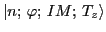
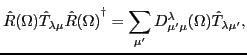
To this end, we first find the self-consistent MF state
and then build a normalized angular-momentum-
and isospin-conserving basis
 by using the projection method:
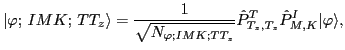 |
(4) |
where
 and
and
 stand for the standard isospin
and angular-momentum projection operators:
stand for the standard isospin
and angular-momentum projection operators:
where,
 is the rotation operator
about the
is the rotation operator
about the  -axis in the isospace,
 is
the Wigner function, and
is
the Wigner function, and
 is the third component
of the total isospin
is the third component
of the total isospin  . As usual,
 is the three-dimensional
rotation operator in space,
is the three-dimensional
rotation operator in space,
 are the
Euler angles,
are the
Euler angles,
 is the Wigner function,
and
is the Wigner function,
and  and
and  denote the angular-momentum components along the
laboratory and intrinsic
denote the angular-momentum components along the
laboratory and intrinsic  -axis, respectively [22,25].
Note that unpaired MF
states
conserve the third isospin component
-axis, respectively [22,25].
Note that unpaired MF
states
conserve the third isospin component
 ; hence, the one-dimensional isospin projection suffices.
The set of states (4) is, in general, overcomplete because
the quantum number is not conserved. This difficulty is overcome
by selecting first the subset of linearly independent states
known as collective space [22], which
is spanned, for each  and
and  , by the so-called natural states
 [26,27].
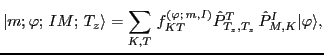
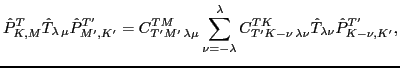
The entire Hamiltonian - including
the ISB terms - is rediagonalized in the collective space, and the resulting
eigenfunctions are:
[26,27].
The entire Hamiltonian - including
the ISB terms - is rediagonalized in the collective space, and the resulting
eigenfunctions are:
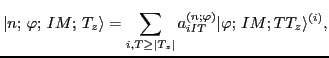 |
(7) |
where the index  labels the eigenstates in ascending order
according to their energies. The amplitudes
labels the eigenstates in ascending order
according to their energies. The amplitudes
 define the degree of isospin mixing through the so-called isospin-mixing
coefficients (or isospin impurities), determined for a given th eigenstate as:
define the degree of isospin mixing through the so-called isospin-mixing
coefficients (or isospin impurities), determined for a given th eigenstate as:
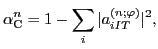 |
(8) |
where the sum of norms
corresponds to the isospin dominating in the wave function
 .
.
One of the advantages of the projected DFT as compared to the
shell-model-based approaches [28,3] is that it allows
for a rigorous quantum-mechanical evaluation of the Fermi matrix element
using the bare isospin operators:
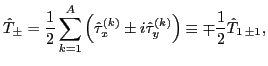 |
(9) |
where
 denotes the rank-one covariant
one-body spherical-tensor operators in the isospace, see the discussion in
Ref. [29,30]. Indeed,
noting that each
denotes the rank-one covariant
one-body spherical-tensor operators in the isospace, see the discussion in
Ref. [29,30]. Indeed,
noting that each  th eigenstate (7) can be uniquely decomposed
in terms of the original basis states (4),
th eigenstate (7) can be uniquely decomposed
in terms of the original basis states (4),
 |
(10) |
with microscopically determined mixing coefficients
 ,
the expression for the Fermi matrix element between the parent state
,
the expression for the Fermi matrix element between the parent state
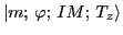 and
daughter state
and
daughter state
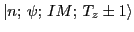 can be written as:
 |
|
|
|
 |
|
|
(11) |
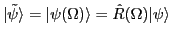
where tilde indicates the Slater determinant rotated in space:
 .
The matrix element appearing on the right-hand side of Eq. (11)
can be expressed through the transition densities that are basic building blocks
of the multi-reference DFT [31,32,33,24].
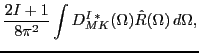
Indeed, with the aid of the identity
.
The matrix element appearing on the right-hand side of Eq. (11)
can be expressed through the transition densities that are basic building blocks
of the multi-reference DFT [31,32,33,24].
Indeed, with the aid of the identity
| |
 |
 |
(12) |
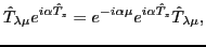
which results from the general transformation rule for spherical tensors under rotations
or isorotations,
 |
(13) |
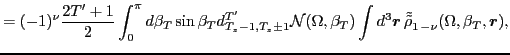
the matrix element entering Eq. (11) can be expressed as:
| |
|
 |
(14) |
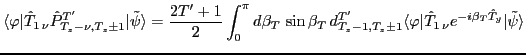
For unpaired Slater determinants considered here,
the double integral over the isospace Euler angles in Eq. (11) can be
further reduced
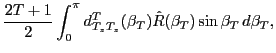
to a one-dimensional integral over the angle  using the identity
 |
(15) |
which is the one-dimensional version of the transformation rule (13) valid for
rotations around the  axis in the isospace. The final expression
for the matrix element in Eq. (14) reads:
axis in the isospace. The final expression
for the matrix element in Eq. (14) reads:
 |
|
|
|
 |
|
|
(16) |
where
 is
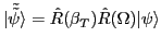
the isovector transition density, and the double-tilde sign indicates
that the right Slater determinant used to calculate this density
is rotated both in space as well as in isospace:
is
the isovector transition density, and the double-tilde sign indicates
that the right Slater determinant used to calculate this density
is rotated both in space as well as in isospace:
 . The symbol
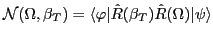 denotes the overlap kernel.
Since the natural states have good isospin,
the states (7) are free from spurious
isospin mixing. Moreover, since the isospin projection is applied to self-consistent
MF solutions, our model accounts for a subtle balance
between the long-range Coulomb polarization,
which tends to make proton and neutron wave functions different,
and the short-range nuclear attraction, which
acts in an opposite way. The long-range polarization
affects globally all s.p. wave functions.
Direct inclusion of this effect in open-shell heavy nuclei is possible essentially only within
the DFT, which is the only no-core microscopic
framework that can be used there.
Recent experimental
data on the isospin impurity deduced in  Zr from the giant dipole
resonance
Zr from the giant dipole
resonance  -decay studies [34] agree well with the
impurities calculated using isospin-projected DFT based on modern Skyrme-force
parametrizations [23,17]. This further demonstrates
that the isospin-projected DFT is capable of capturing the essential piece
of physics associated with the isospin mixing.
-decay studies [34] agree well with the
impurities calculated using isospin-projected DFT based on modern Skyrme-force
parametrizations [23,17]. This further demonstrates
that the isospin-projected DFT is capable of capturing the essential piece
of physics associated with the isospin mixing.
Next: The choice of Skyrme
Up: The model
Previous: The model
Jacek Dobaczewski
2012-10-19