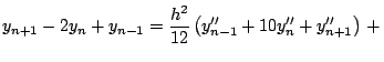
The Numerov (Cowell) method [23] is the standard
technique for a precise integration of second-order differential
equations; here we only give some details pertaining to
its application to the system of two HFB equations (34).
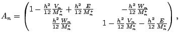
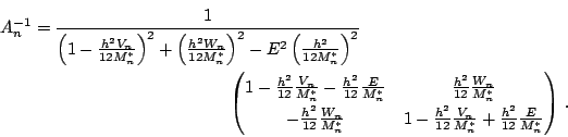
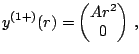
Let function ![]() be the solution of the differential equation
be the solution of the differential equation
 |
(62) |
 |
(65) |
 and and |
(66) |
The eigen energies are found by integrating two linearly
independent solutions,
![]() and
and
![]() ,
from the origin to a given point
,
from the origin to a given point ![]() , called the matching point.
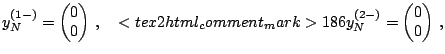
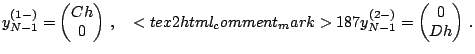
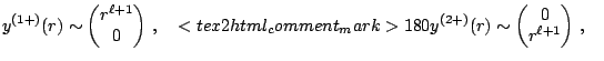
These two solutions are selected by imposing that either
the first or the second component of the quasiparticle wave function
vanishes near the origin, i.e.,
, called the matching point.
These two solutions are selected by imposing that either
the first or the second component of the quasiparticle wave function
vanishes near the origin, i.e.,
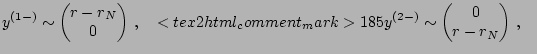
Next, another two linearly
independent solutions,
![]() and
and
![]() , are found
by the backward integration from the wall of the box
, are found
by the backward integration from the wall of the box
![]() to
to ![]() , again imposing that either
the first or the second component of the quasiparticle wave function
vanishes near
, again imposing that either
the first or the second component of the quasiparticle wave function
vanishes near ![]() for the Dirichlet boundary conditions, i.e.,
for the Dirichlet boundary conditions, i.e.,
The boundary conditions (69)-(70)
and (72)-(73)
determine the initial values
![]() and
and
![]() , respectively, needed to start the Numerov iterations of (65).
Obviously, a correct limit should be taken when calculating
values of
, respectively, needed to start the Numerov iterations of (65).
Obviously, a correct limit should be taken when calculating
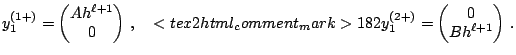
values of ![]() from Eq. (64). It turns out that one
obtains
from Eq. (64). It turns out that one
obtains ![]() =0 for all partial waves except
=0 for all partial waves except ![]() , which is the
case that deserves a little more attention. For example,
focusing our attention on one of the solutions,
, which is the
case that deserves a little more attention. For example,
focusing our attention on one of the solutions,
 |
(73) |
 |
(74) |
The eigenenergies are found by requiring that the full
solution
![]() and its first derivative are continuous at
and its first derivative are continuous at ![]() (see for example [24]).
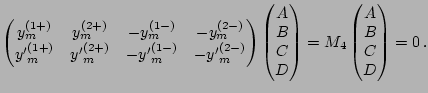
This matching conditions read
(see for example [24]).
This matching conditions read
For vanishing determinant, Eq. (76) is used
to determine three of the multiplicative
constants in terms of the fourth one.
This is done by extracting a ![]() matrix
matrix ![]() out
of
out
of ![]() and inverting it.
Among the four possible choices one may have for
and inverting it.
Among the four possible choices one may have for ![]() we retain
the one for which the product
we retain
the one for which the product
![]() is
closest to unity. Finally, the fourth multiplicative
constant is fixed by the normalization condition of the wave
function.
is
closest to unity. Finally, the fourth multiplicative
constant is fixed by the normalization condition of the wave
function.
When approaching the self-consistent solution, the eigenenergies do not change very much between two consecutive Bogolyubov iterations. We take advantage of this fact by keeping in memory the intervals where the solutions are located and using them as initial guesses for the next iteration. This results in finding solutions for eigenenergies faster and faster as we get closer to the converged self-consistent state.
 o
o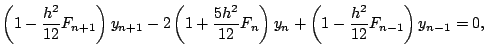
![$\displaystyle \left\{\begin{matrix}G_{n+1} =& 12 y_n - 10 G_n - G_{n-1}\,, \hfill\\ [1.5mm] \hfill y_{n+1} =& A_{n+1}^{-1}G_{n+1}\,. \hfill\\ \end{matrix}\right.$](img230.png)
 for
for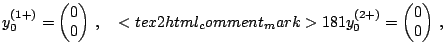
 for
for