Hartree-Fock-Bogoliubov Method

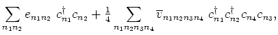
A two-body Hamiltonian of a system of fermions can be expressed in terms of a set of annihilation and creation operators $(c,c^{\dagger })$:

$$H = \sum_{n_{1}n_{2}}e_{n_{1}n_{2}}~c_{n_{1}}^{\dagger }c_{n_{2}} +{\... ...{1}n_{2}n_{3}n_{4}}~c_{n_{1}}^{\dagger }c_{n_{2}}^{\dagger }c_{n_{4}}c_{n_{3}},$$ (1)

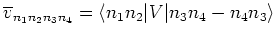where $\overline{v}_{n_{1}n_{2}n_{3}n_{4}}=\langle n_{1}n_{2}\vert V\vert n_{3}n_{4}-n_{4}n_{3}\rangle$ are anti-symmetrized two-body interaction matrix-elements. In the HFB method, the ground-state wave function $\vert\Phi \rangle$ is defined as the quasiparticle vacuum $\alpha _{k}\vert\Phi \rangle =0$, where the quasiparticle operators $(\alpha ,\alpha^{\dagger })$ are connected to the original particle operators via the linear Bogoliubov transformation

$$\quad \quad \alpha_{k} = \sum_{n}\left( U_{nk}^{\ast }c_{n}+V_{nk}^{\ast }c_{n}^{\dagger }... ...lpha_{k}^{\dagger } =\sum_{n}\left( V_{nk}c_{n}+U_{nk}c_{n}^{\dagger }\right) ,$$ (2)

which can be rewritten in the matrix form as

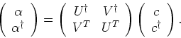$$\left( \begin{array}{c} \alpha \\ \alpha^{\dagger } \end{ar... ...eft( \begin{array}{c} c \\ c^{\dagger } \end{array}\right) .$$ (3)

Matrices $U$ and $V$ satisfy the relations:

$$U^{\dagger }U+V^{\dagger }V=I,~~~UU^{\dagger }+V^{\ast }V^{T}=I,~~~U^{T}V+V^{T}U=0,~~~UV^{\dagger }+V^{\ast }U^{T}=0.$$ (4)

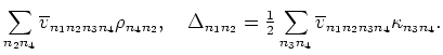
In terms of the normal $\rho$ and pairing $\kappa$ one-body density matrices, defined as

$$\rho_{nn^{\prime }}~=~\langle \Phi \vert c_{n^{\prime }}^{\d... ...me }}c_{n}\vert\Phi \rangle=(V^{\ast }U^{T})_{nn^{\prime }} ,$$ (5)

the expectation value of the Hamiltonian (1) is expressed as an energy functional

$$E[\rho ,\kappa ] = \frac{\langle \Phi \vert H\vert\Phi \rangle }{\langle \Phi \vert\... ...right] -{\textstyle{\frac{1}{2}}}{\rm Tr} \left[ \Delta \kappa^{\ast }\right] ,$$ (6)

where

$$\Gamma_{n_{1}n_{3}} = \sum_{n_{2}n_{4}}\overline{v}_{n_{1}n_{2}n_{3}n_{4}} \rho_{n_{4}n... ...}{2}}}\sum_{n_{3}n_{4}}\overline{v} _{n_{1}n_{2}n_{3}n_{4}}\kappa_{n_{3}n_{4}}.$$ (7)

Variation of energy (6) with respect to $\rho$ and $\kappa$ results in the HFB equations:

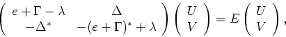$$\left( \begin{array}{cc} e+\Gamma -\lambda & \Delta \\ -\De... ...\right) =E\left( \begin{array}{c} U \\ V \end{array}\right) ,$$ (8)

where the Lagrange multiplier $\lambda$ has been introduced to fix the correct average particle number.

It should be stressed that the modern energy functionals (6) contain terms that cannot be simply related to some prescribed effective interaction, see e.g., Ref. [27,28] for details. In this respect the functional (6) should be considered in the broader context of the energy density functional theory.