next up previous
Next: Potentials in the spherical Up: The NLO potentials, fields, Previous: Spherical HO basis


Densities in the spherical HO basis

For any density matrix one can always perform a multipole expansion. This strategy fits very well our applications to the spherical HF solutions, where only the monopole component of the density matrix is nonzero, and to the RPA applications in spherical nuclei, where all multipole excitations separate from one another. Therefore, 
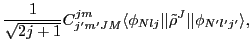
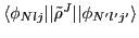
in what follows we consider the density matrix of multipolarity $J$ in the form given by the Wigner-Eckart theorem:

$\displaystyle \tilde{\rho}^{JM}_{Nljm,N'l'j'm'}$ $\textstyle =$ $\displaystyle \frac{1}{\sqrt{2j+1}} C^{jm}_{j'm'JM} \langle\phi_{Nlj}\vert\vert\tilde{\rho}^{J}\vert\vert\phi_{N'l'j'}\rangle ,$ (88)

and depending on its reduced matrix elements $\langle\phi_{Nlj}\vert\vert\tilde{\rho}^{J}\vert\vert\phi_{N'l'j'}\rangle$ 
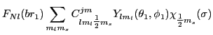
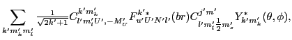
Then, the non-local densities can be expressed in terms of the spherical HO wave functions (79) as
$\displaystyle \tilde{\rho}^{J''M''}_{v\mu}(\vec{r}_1,\vec{r}_2)\!\!\!\!$ $\textstyle =$ $\displaystyle \sum_{{Nljm\sigma}\atop{N'l'j'm'\sigma'}} \!\!\!\!
\phi_{Nljm}(\v...
...'l'j'm'}(\vec{r}_2,\sigma')
\langle\sigma'\vert\sigma_{v\mu}\vert\sigma\rangle,$  

that is,
$\displaystyle \tilde{\rho}^{J''M''}_{v\mu}(\vec{r}_1,\vec{r}_2)\!\!\!\!$ $\textstyle =$ $\displaystyle \sum_{{Nljm\sigma}\atop{N'l'j'm'\sigma'}} \!\!\!\! b^{3}
e^{-\fr...
...r_1)^2-\frac{1}{2}(br_2)^2}
\langle\sigma'\vert\sigma_{v\mu}\vert\sigma\rangle$  
  $\textstyle \times$ $\displaystyle F_{Nl}(br_1)
\sum_{m_lm_s}C^{jm}_{lm_l{\textstyle{\frac{1}{2}}}m_s}Y_{lm_l}(\theta_1,\phi_1)\chi_{{\textstyle{\frac{1}{2}}}m_s}(\sigma)$  
  $\textstyle \times$ $\displaystyle {\textstyle{\frac{1}{\sqrt{2j+1}}}} C^{jm}_{j'm'J''M''} \langle\phi_{Nl j}\vert\vert\tilde{\rho}^{J''}\vert\vert\phi_{N'l'j'}\rangle$  
  $\textstyle \times$ $\displaystyle F_{N'l'}(br_2)
\sum_{m'_lm'_s}C^{j'm'}_{l'm'_l{\textstyle{\frac{1...
..._s}Y^*_{l'm'_l}(\theta_2,\phi_2)\chi_{{\textstyle{\frac{1}{2}}}m'_s}(\sigma') .$ (89)

We can now replace the spin coordinates by the spin projections,
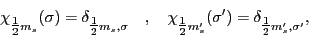
\begin{displaymath}
\chi_{{\textstyle{\frac{1}{2}}}m_s}(\sigma) = \delta_{{\text...
..._s}(\sigma') = \delta_{{\textstyle{\frac{1}{2}}}m'_s,\sigma'},
\end{displaymath} (90)

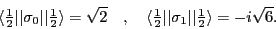
and we can use the Wigner-Eckart theorem for the Pauli matrices,
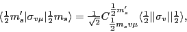
\begin{displaymath}
\langle{\textstyle{\frac{1}{2}}}m'_s\vert\sigma_{v\mu}\vert{...
...ert\vert\sigma_{v}\vert\vert{\textstyle{\frac{1}{2}}}\rangle ,
\end{displaymath} (91)

with
\begin{displaymath}
\langle{\textstyle{\frac{1}{2}}}\vert\vert\sigma_{0}\vert\ve...
...a_{1}\vert\vert{\textstyle{\frac{1}{2}}}\rangle = -i\sqrt{6} .
\end{displaymath} (92)

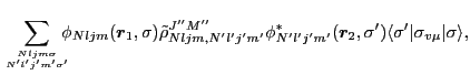
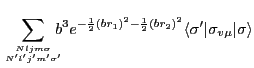
After inserting the nonlocal density (93) into the expression for local densities (76), and after acting with derivatives on spherical wave functions, as in Eqs. (81) and (82), we obtain
$\displaystyle \tilde{\rho}^{uUu'U'W,J''M''}_{vJ'M'}(\vec{r})
\!\!\!\!$ $\textstyle =$ $\displaystyle \sum_{M_W\mu} C^{J'M'}_{WM_Wv\mu}
\sum_{M_UM'_U}C^{WM_W}_{UM_UU'M'_U} (-1)^{U'-M'_U}$  
  $\textstyle \times$ $\displaystyle \sum_{{Nljmm_s}\atop{N'l'j'm'm'_s}} \!\!\!\! b^{3+u+u'} e^{-(br)^...
...yle{\frac{1}{2}}}\vert\vert\sigma_{v}\vert\vert{\textstyle{\frac{1}{2}}}\rangle$  
  $\textstyle \times$ $\displaystyle \sum_{km_km_l}{\textstyle{\frac{1}{\sqrt{2k+1}}}}
C^{km_k}_{lm_l...
...F^{k}_{uUNl}(br)
C^{jm}_{lm_l{\textstyle{\frac{1}{2}}}m_s}Y_{km_k}(\theta,\phi)$  
  $\textstyle \times$ $\displaystyle {\textstyle{\frac{1}{\sqrt{2j+1}}}} C^{jm}_{j'm'J''M''} \langle\phi_{Nl j}\vert\vert\tilde{\rho}^{J''}\vert\vert\phi_{N'l'j'}\rangle$ (93)
  $\textstyle \times$ $\displaystyle \sum_{k'm'_km'_l}{\textstyle{\frac{1}{\sqrt{2k'+1}}}}
C^{k'm'_k}...
...}(br)
C^{j'm'}_{l'm'_l{\textstyle{\frac{1}{2}}}m'_s}Y^*_{k'm'_k}(\theta,\phi) ,$  

where, by using the phase convention $D^{(2)}_{u'U'M'_U}=(-1)^{U'-M'_U}D^{(2)*}_{u'U',-M'_U}$, we have introduced the complex conjugation into the derivative operator (31).

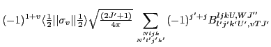
After a lengthy but straightforward derivation presented in B, we obtain the following result:

$\displaystyle \tilde{\rho}^{uUu'U'W,J''M''}_{vJ'M'}(\vec{r})
\!\!\!\!$ $\textstyle =$ $\displaystyle \sum_{TM_T} \tilde{\rho}^{uUu'U'W,J''}_{vTJ'}(br) e^{-(br)^2}
C^{TM_T}_{J'M'J''M''} Y_{TM_T}(\theta,\phi) ,$ (94)

for the radial form factors $\tilde{\rho}^{uUu'U'W,J''}_{vTJ'}(br)$ given by:
$\displaystyle \tilde{\rho}^{uUu'U'W,J''}_{vTJ'}(br) \!\!\!\!$ $\textstyle =$ $\displaystyle (-1)^{1+v}
\langle{\textstyle{\frac{1}{2}}}\vert\vert\sigma_{v}\v...
...{4\pi}}}}
\sum_{{Nljk}\atop{N'l'j'k'}}(-1)^{j'+j} B^{ljkU,WJ''}_{l'j'k'U',vTJ'}$  
$\displaystyle $ $\textstyle \times$ $\displaystyle b^{3+u+u'}F^{k}_{uUNl}(br)
\langle\phi_{Nl j}\vert\vert\tilde{\rho}^{J''}\vert\vert\phi_{N'l'j'}\rangle
F^{k'}_{u'U'N'l'}(br) ,$ (95)

where
$\displaystyle B^{ljkU,WJ''}_{l'j'k'U',vTJ'} \!\!\!\!$ $\textstyle =$ $\displaystyle (-1)^{k}(-1)^{T}(-1)^{U-W}C^{T0}_{k0k'0}
{\textstyle{\sqrt{\frac{(2k+1)(2k'+1)(2W+1)(2j+1)(2j'+1)}{(2T+1)}}}}$  
  $\textstyle \times$ $\displaystyle \sum_{T'} (-1)^{T'}(2T'+1)$  
  $\textstyle \times$ $\displaystyle \left\{\begin{array}{rrr} j & j' & J'' \\
{\textstyle{\frac{1}...
...}
\left\{\begin{array}{rrr} v & T' & J'' \\
T & J' & W \end{array}\right\} .$ (96)

In view of the fact that only the coefficients $B^{ljkU,WJ''}_{l'j'k'U',vTJ'}$ for $(-1)^{l+k+U}=1$ and $(-1)^{l'+k'+U'}=1$ are required in Eq. (99), we may replace them by coefficients $\tilde{B}^{ljkU,WJ''}_{l'j'k'U',vTJ'}$:
$\displaystyle \tilde{B}^{ljkU,WJ''}_{l'j'k'U',vTJ'} \!\!\!\!$ $\textstyle =$ $\displaystyle (-1)^{l}C^{T0}_{k0k'0}
{\textstyle{\sqrt{\frac{(2k+1)(2k'+1)(2W+1)(2j+1)(2j'+1)}{(2T+1)}}}}$  
  $\textstyle \times$ $\displaystyle \sum_{T'} (2T'+1)$  
  $\textstyle \times$ $\displaystyle \left\{\begin{array}{rrr} {\textstyle{\frac{1}{2}}} & {\textstyle...
...}
\left\{\begin{array}{rrr} v & T' & J'' \\
T & J' & W \end{array}\right\} ,$ (97)

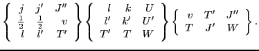
where we have used symmetry properties of 9j symbols under the transposition of rows and columns and transposition with respect to the main diagonal.

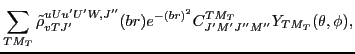
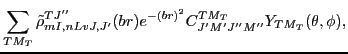
Finally, all secondary densities of Eq. (77) can now be calculated in terms of one compact expression:

$\displaystyle \tilde{\rho}_{mI,nLvJ,J'M'}^{J''M''}(\vec{r})$ $\textstyle =$ $\displaystyle \sum_{TM_T} \tilde{\rho}_{mI,nLvJ,J'}^{TJ''}(br) e^{-(br)^2}
C^{TM_T}_{J'M'J''M''} Y_{TM_T}(\theta,\phi) ,$ (98)

where the radial form factors read
$\displaystyle \tilde{\rho}_{mI,nLvJ,J'}^{TJ''}(br) \!\!$ $\textstyle =$ $\displaystyle \sum_{uUu'U'W} A^{uUu'U'W}_{mI,nLvJ,J'}\,\tilde{\rho}^{uUu'U'W,J''}_{vTJ'}(br) .$ (99)


next up previous
Next: Potentials in the spherical Up: The NLO potentials, fields, Previous: Spherical HO basis
Jacek Dobaczewski 2010-01-30