


Next: Fields
Up: General forms of the
Previous: Building blocks
Potentials
The potential energy to be varied over the wave functions is given in Ref. [4]
and reads
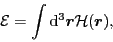 |
(36) |
for
where
 are the coupling constants
and
are the coupling constants
and
 are the primary densities:
![\begin{displaymath}
\rho_{nLvJ}(\vec{r})=\left\{[K_{nL}\rho_v(\vec{r},\vec{r}')]_J \right\}_{\vec{r}'=\vec{r}},
\end{displaymath}](img108.png) |
(38) |
which are built by acting with the relative momentum operators  on the scalar (
 ) and vector (
 ) non-local densities:
Note that the sum in Eq. (38) runs over the indices
ordered in a specific way, defined
in Ref. [4,5],
namely,
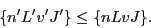 |
(40) |
We first vary  over the densities and then, in Section 3.3, we vary densities
over the wave functions, that is, we begin with
over the densities and then, in Section 3.3, we vary densities
over the wave functions, that is, we begin with
An explicit variation over the primary densities under the differential
operators  can be avoided by first integrating
by parts and recoupling. The recoupling within
a scalar [6] is simple, namely,
can be avoided by first integrating
by parts and recoupling. The recoupling within
a scalar [6] is simple, namely,
Hence, the integration by parts gives:
where we have used Eq. (33), then we changed the names of indices,
and we also used the fact that  is even.
Therefore, the variation under the differential
operators
only gives the transposition of indices
 and the phase. The complete variation of the energy then reads:
where we defined potentials
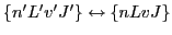
Note that because of the ordering (41),
in Eq. (46)
either the first or the second term is non-zero (for
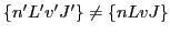 ),
or both terms add up to
),
or both terms add up to
 (for
(for
 ).
).
Next: Fields
Up: General forms of the
Previous: Building blocks
Jacek Dobaczewski
2010-01-30
![$\displaystyle \sum_{{n'L'v'J'}\atop{mI,nLvJ}}
C^{n'L'v'J'}_{mI,nLvJ}\, [\rho_{n'L'v'J'}(\vec{r})[D_{mI}\rho_{nLvJ}(\vec{r})]_{J'}]_0$](img104.png)
![$\displaystyle \sum_{{n'L'v'J'M'}\atop{mI,nLvJ}}
\!\!\!
C^{n'L'v'J'}_{mI,nLvJ}
{...
...t{2J'+1}}}}
\, \rho_{n'L'v'J'M'}(\vec{r})[D_{mI}\rho_{nLvJ}(\vec{r})]_{J',-M'},$](img105.png)
![$\displaystyle \sum_{{n'L'v'J'}\atop{mI,nLvJ}} (-1)^{J'+I-J}
C^{n'L'v'J'}_{mI,nLvJ}\, [\rho_{nLvJ}(\vec{r})[D^T_{mI}\rho_{n'L'v'J'}(\vec{r})]_J]_0$](img120.png)
![$\displaystyle \sum_{{n'L'v'J'}\atop{mI,nLvJ}} (-1)^{m+J'+I-J}
C^{n'L'v'J'}_{mI,nLvJ}\, [\rho_{nLvJ}(\vec{r})[D_{mI}\rho_{n'L'v'J'}(\vec{r})]_J]_0$](img121.png)
![$\displaystyle \sum_{{n'L'v'J'}\atop{mI,nLvJ}} (-1)^{J-J'}
C^{nLvJ}_{mI,n'L'v'J'}\, [\rho_{n'L'v'J'}(\vec{r})[D_{mI}\rho_{nLvJ}(\vec{r})]_{J'}]_0 ,$](img122.png)
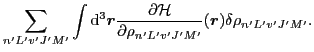
![$\displaystyle \sum_{n'L'v'J'}\int {\rm d}^3\vec{r}[\delta\rho_{n'L'v'J'}\tilde{U}_{n'L'v'J'}(\vec{r})]_0 ,$](img126.png)
![$\displaystyle \sum_{mI,nLvJ}\!\!
\left\{C^{n'L'v'J'}_{mI,nLvJ}+(-1)^{J-J'}C^{nLvJ}_{mI,n'L'v'J'}\right\}
[D_{mI}\rho_{nLvJ}(\vec{r})]_{J'M'}.$](img128.png)