Next: Numerical applications: the isospin
Up: Isospin mixing of isospin-projected
Previous: Introduction
Theoretical formalism: isospin restoration and Coulomb
rediagonalization scheme
The first step and the starting point of our approach is the determination
of the isospin-symmetry-broken
single-particle (s.p.) Slater determinant
 calculated by using the Hartree-Fock (HF) theory including the isospin-invariant Skyrme
(
calculated by using the Hartree-Fock (HF) theory including the isospin-invariant Skyrme
( ) and the isospin-symmetry-breaking Coulomb (
 )
interactions:
)
interactions:
 |
(1) |
The isospace-deformed state
admixes higher isospin components  :
:
 |
(2) |
where  and
and  are the total isospin and its third component,
respectively,
are the total isospin and its third component,
respectively,  labels all other quantum numbers
pertaining to the
state, and the coefficients
labels all other quantum numbers
pertaining to the
state, and the coefficients
 are such that
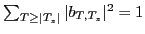 .
.
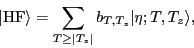
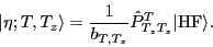
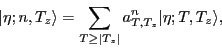
In the second step we create the good-isospin states
 by projecting them out from the Slater determinant
:
by projecting them out from the Slater determinant
:
 |
(3) |
In the following, we denote the mixing coefficients and average energies
 :
:
 |
(4) |
as being obtained before rediagonalization.
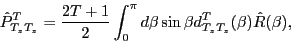
In the above formulae,
 denotes the conventional[11] SO(3) projection
operator reduced to one dimension due to the quantum number
conservation, that is:
denotes the conventional[11] SO(3) projection
operator reduced to one dimension due to the quantum number
conservation, that is:
 |
(5) |
where
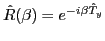 denotes active-rotation operator by the Euler angle
  in
the isospace and
in
the isospace and
 is the Wigner
 -function[12].
In the third step we mix the projected states,
 |
(6) |
and determine the mixing coefficients  by diagonalizing
Hamiltonian (1) in the space of projected states,
by diagonalizing
Hamiltonian (1) in the space of projected states,
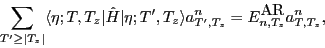 |
(7) |
where  enumerates the obtained eigenstates.
In the following, we denote the mixing coefficients and eigenenergies
enumerates the obtained eigenstates.
In the following, we denote the mixing coefficients and eigenenergies
 as being obtained after rediagonalization.
The lowest-energy solution, for
as being obtained after rediagonalization.
The lowest-energy solution, for  , corresponds to the isospin mixing in the
ground state.
, corresponds to the isospin mixing in the
ground state.
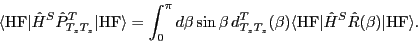
The Skyrme Hamiltonian,  , is an isoscalar operator; hence, it contributes
only to the diagonal matrix elements of the Hamiltonian (1),
, is an isoscalar operator; hence, it contributes
only to the diagonal matrix elements of the Hamiltonian (1),
 , which can be obtained from:
 |
(8) |
Similarly, calculation of the diagonal and non-diagonal
matrix elements of the Coulomb interaction,
 ,
can be efficiently performed after decomposing
,
can be efficiently performed after decomposing  into the isoscalar,
 , isovector,
 , and
isotensor,
, and
isotensor,
 , components,
and by making use of the SO(3) transformation rules for the
spherical tensors under rotations in the isospace[12].
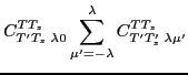
In the particular case of one-dimensional projection we deal with in
this work, all matrix elements of axial spherical tensors
reduce to one-dimensional integrals over the Euler angle :
, components,
and by making use of the SO(3) transformation rules for the
spherical tensors under rotations in the isospace[12].
In the particular case of one-dimensional projection we deal with in
this work, all matrix elements of axial spherical tensors
reduce to one-dimensional integrals over the Euler angle :
where
 and
and
 denote standard
Clebsch-Gordan coefficients.
The Skyrme-Hamiltonian and Coulomb-interaction kernels,
denote standard
Clebsch-Gordan coefficients.
The Skyrme-Hamiltonian and Coulomb-interaction kernels,
 and
and
 ,
respectively, can be evaluated by using expressions for the standard
diagonal kernels[13] (
,
respectively, can be evaluated by using expressions for the standard
diagonal kernels[13] ( ) and replacing there the
isoscalar and isovector densities and currents with the so-called
transition densities and currents. Exact direct and exchange kernels
of the Coulomb interaction can be evaluated by using methods outlined
in Refs.[14,15,16].
) and replacing there the
isoscalar and isovector densities and currents with the so-called
transition densities and currents. Exact direct and exchange kernels
of the Coulomb interaction can be evaluated by using methods outlined
in Refs.[14,15,16].
Next: Numerical applications: the isospin
Up: Isospin mixing of isospin-projected
Previous: Introduction
Jacek Dobaczewski
2009-04-13