QRPA method

In the present study, we solve the QRPA equations by using the iterative Arnoldi method, implemented in Ref. [22]. It provides us with an extremely efficient and fast way to solve the QRPA equations. The QRPA equations are well known [24,25] and have been recently reviewed in the context of the finite amplitude method [26]. Therefore, here we only give a brief resumé of basic equations, by presenting their particularly useful and compact form.

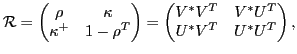
Basic dynamical variables of the QRPA method are given by the generalized density matrix ${\cal R}$,

$${\cal R} = \begin{pmatrix}\rho & \kappa \\ \kappa^{+} & 1-\rho^{T... ...nd{pmatrix} = \begin{pmatrix}V^*V^T & V^*U^T \\ U^*V^T & U^*U^T \end{pmatrix} ,$$ (1)

corresponding to mean-field Hamiltonian ${\cal H}= \partial {\cal E}/ \partial {\cal R}$,

$${\cal H} = \begin{pmatrix}h-\lambda & \Delta \\ \Delta^{+} & -h^{*}+\lambda \end{pmatrix} .$$ (2)

The standard HFB equations that define amplitudes $U$ and $V$ read

$$\begin{pmatrix}h-\lambda & \Delta \\ \Delta^{+} & -h^{*}+\lambda ... ...x}U & V^* \\ V & U^* \end{pmatrix} \begin{pmatrix}E & 0 \\ 0 & -E \end{pmatrix}$$ (3)

where the diagonal matrix $E$ contains positive quasiparticle energies. Then the quasiparticle ($\chi$) and quasihole ($\varphi$) states are given by columns of eigen-vectors:

$$\varphi := \begin{pmatrix}V^* \\ U^* \end{pmatrix}, \hspace{2.0cm} \chi := \begin{pmatrix}U \\ V \end{pmatrix},$$ (4)

that is,

$${\cal H} \varphi = - \varphi E, \hspace{2.0cm} {\cal H} \chi = \chi E .$$ (5)

The vibrational time-dependent HFB state $\vert\Psi(t)\rangle$,

$$\vert\Psi(t)\rangle = \vert\Psi\rangle + ^{i\omega t} \vert\tilde{\Psi}\rangle ,$$ (6)

where $\vert\tilde{\Psi}\rangle$ is a small-amplitude correction, leads to the time-dependent density matrix,

$${\cal R}(t) = {\cal R} + ^{i\omega t} \tilde{\cal R} + ^{-i\omega t} \tilde{\cal R}^{+}$$ (7)

and time-dependent mean field ${\cal H}(t)$,

$${\cal H}(t) = {\cal H} + ^{i\omega t} \tilde{\cal H} + ^{-i\omega t} \tilde{\cal H}^{+} .$$ (8)

After a linearization of fields in the time-dependent Hamiltonian, one obtains the QRPA equations in a simple form,

$$-\hbar \omega \tilde{\cal R} = [{\cal H},\tilde{\cal R}] + [\tilde{\cal H},{\cal R}].$$ (9)

In this approach, states in Eq. (6) play a role of Kohn-Sham-like wave functions, which serve the purpose of generating generalized density matrices ${\cal R}(t)$ only. Neither $\vert\Psi\rangle$ represents a correct ground state of the system nor $\vert\tilde{\Psi}\rangle$ represents that of an excited vibrational state. However, the amplitude $\tilde{\cal R}$, which constitutes the fundamental degree of freedom of the QRPA method, does represent a fair approximation to the transition density matrix between both states of the system. It then allows for calculating matrix elements of arbitrary one-body operators between the ground state and vibrational state, which is the primary goal of the QRPA approach.

Equation (9) constitutes the base for our solution of the QRPA equations in terms of the iterative Arnoldi method. Indeed, since the mean-field amplitude $\tilde{\cal H}$ depends linearly on the density amplitude $\tilde{\cal R}$, Eq. (9) constitutes an eigen-equation determining $\tilde{\cal R}$ and $\hbar \omega$. However, the matrix to be diagonalized, that is the QRPA matrix, does not have to be explicitly determined. To obtain the entire QRPA strength function, it is enough to start from a pivot amplitude and repeatedly act on it with the expression on the right-hand side [22]. In each iteration, one only has to calculate the mean-field amplitude $\tilde{\cal H}$ corresponding to the current density amplitude $\tilde{\cal R}$, which is an easy task. The pivot can be freely chosen to optimally suit the calculation. It can for example be random, a QRPA eigen-phonon or be constructed from an external field. In this work we construct the pivot from the monopole transition operator. This approach is fundamentally different than that used within the FAM of Ref. [26], where an external field is used throughout the calculation and Eq. (9) has to be iterated for all values of frequencies $\omega$.

Since both stationary ( ${\cal R}^2 = {\cal R}$) and time-dependent, ( ${\cal R}^2(t) = {\cal R}(t)$) density matrices are projective, the QRPA amplitude $\tilde{\cal R}$ has vanishing matrix elements between the quasihole and between the quasiparticle states, that is,

$$\varphi^{+} \tilde{\cal R} \varphi = \chi^{+} \tilde{\cal R} \chi = 0 .$$ (10)

Therefore, $\tilde{\cal R}$ is solely defined through the antisymmetric amplitude matrices $\tilde{Z}$ and $\tilde{Z}'^{+}$ defined as

$$\tilde{Z} = - \tilde{Z}^{T} = \chi^{+} \tilde{\cal R} \varphi ,$$

$$\tilde{Z}'^{+} = - \tilde{Z}'^{*} = \varphi^{+} \tilde{\cal R} \chi .$$ (11)

Explicitly, amplitudes $\tilde{Z}$ and $\tilde{Z}'^{+}$ read

$$\tilde{Z} = U^{+} \tilde{\rho} V^{*} + U^{+} \tilde{\kappa} U^{*} + V^{+} \tilde{\kappa}'^{+} V^{*} - V^{+} \tilde{\rho}^{T} U^{*} ,$$

$$\tilde{Z}'^{+} = V^{T} \tilde{\rho} U + V^{T} \tilde{\kappa} V + U^{T} \tilde{\kappa}'^{+} U - U^{T} \tilde{\rho}^{T} V .$$ (12)

Within such a formalism, the QRPA equations (9) can be expressed as

$$-\hbar \omega \tilde{Z} = E \tilde{Z} + \tilde{Z} E + \tilde{W} ,$$

$$\hbar \omega \tilde{Z}'^{+} = E \tilde{Z}'^{+} + \tilde{Z}'^{+} E + \tilde{W}'^{+} ,$$ (13)

where the field amplitudes $\tilde{W}$ and $\tilde{W}'^{+}$ are defined as

$$\tilde{W} = - \tilde{W}^{T} = \chi^{+} \tilde{\cal H} \varphi ,$$

$$\tilde{W}'^{+} = - \tilde{W}'^{*} = \varphi^{+} \tilde{\cal H} \chi ,$$ (14)

or explicitly,

$$\tilde{W} = U^{+} \tilde{h} V^{*} + U^{+} \tilde{\Delta} U^{*} + V^{+} \tilde{\Delta}'^{+} V^{*} - V^{+} \tilde{h}^{T} U^{*} ,$$

$$\tilde{W}'^{+} = V^{T} \tilde{h} U + V^{T} \tilde{\Delta} V + U^{T} \tilde{\Delta}'^{+} U - U^{T} \tilde{h}^{T} V .$$ (15)

We can also invert Eq. (12) and obtain transition densities $\tilde{\rho}$, $\tilde{\kappa}$, and $\tilde{\kappa}'^{+}$ expressed in terms of amplitudes $\tilde{Z}$ and $\tilde{Z}'^{+}$, that is,

$$\tilde{\rho} = U \tilde{Z} V^{T} + V^* \tilde{Z}'^{+} U^{+} ,$$

$$\tilde{\kappa} = U \tilde{Z} U^{T} + V^* \tilde{Z}'^{+} V^{+} ,$$

$$\tilde{\kappa}'^{+} = V \tilde{Z} V^{T} + U^* \tilde{Z}'^{+} U^{+} .$$ (16)

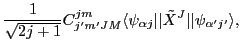
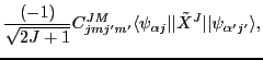
Finally, we can reduce the above QRPA formalism to spherical symmetry used in the present study. Then, the vibrating amplitude of Eq. (6) has good angular-momentum quantum numbers $JM$, that is, $\vert\tilde{\Psi}\rangle\equiv\vert\tilde{\Psi}^{JM}\rangle$ and hence all the QRPA amplitudes pertain to the given preselected channel $JM$, while the ground state $\vert\Psi\rangle$ is spherical. As a consequence, as dictated by the angular-momentum algebra, only specific spherical single-particle states are coupled by the QRPA amplitudes, which can be expressed through the Wigner-Eckart theorem and reduced matrix elements as

$$\tilde{X}^{JM}_{\alpha jm,\alpha'j'm'} =\!\! \frac{1}{\sqrt{2j+1}} C^{jm}_{j'm'JM} \langle\psi_{\alpha j}\vert\vert\tilde{X}^{J}\vert\vert\psi_{\alpha'j'}\rangle ,$$ (17)

where $\tilde{X}$ stands for amplitudes $\tilde{\rho}$ or $\tilde{h}$, and

$$\tilde{X}^{JM}_{\alpha jm,\alpha'j'm'} =\!\! \frac{(-1)}{\sqrt{2J+1}} C^{JM}_{jmj'm'} \langle\psi_{\alpha j}\vert\vert\tilde{X}^{J}\vert\vert\psi_{\alpha'j'}\rangle ,$$ (18)

$$\tilde{X}'{}^{+JM}_{\alpha jm,\alpha'j'm'} =\!\! \frac{(-1)^{J-M}}{\sqrt{2J+1}} C^{J,-M}_{jmj'm'} \langle\psi_{\alpha j}\vert\vert\tilde{X}'{}^{+J}\vert\vert\psi_{\alpha'j'}\rangle ,$$ (19)

where $\tilde{X}$ stands for amplitudes $\tilde{\kappa}$, $\tilde{\Delta}$, $\tilde{Z}$, or $\tilde{W}$. In these expressions, we have used the standard quantum numbers $\alpha jm$ of spherical single-particle states.

Spurious QRPA mode appears in the $0^+$ QRPA calculations. In a self-consistent full QRPA diagonalization, the spurious mode decouples from the physical QRPA modes and appears at zero energy. In the Arnoldi method, this separation does not happen unless we make the full Arnoldi diagonalization, which usually is not feasible.

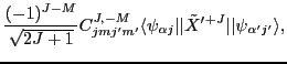
To prevent the mixing of physical QRPA excitations with the spurious $0^+$ mode, before the Arnoldi iteration we create the spurious-mode QRPA amplitudes and its associated conjugate-state (boost-mode) QRPA amplitudes. The spurious $0^+$ mode amplitudes follow from the particle number operator and have the form,

$$\tilde{P}^{00} = U^+ V^* , \quad \tilde{P}'^{+00} = V^T U.$$ (20)

The $0^+$ boost mode is generated by making an additional HFB calculation whose chemical potentials $\lambda_\tau$ and average particle numbers are slightly shifted from the ground state values, producing a perturbed state $\vert {\rm HFB}_2\rangle$. The boost-mode amplitudes are calculated by using Thouless theorem as,

$$\tilde{R}^{00}_{\alpha jm, \alpha' j'm'} = \frac{ \langle {\rm HFB}_2\vert a^+_{\alpha jm} a^+_{\alpha'j'm'} \vert {\rm HFB}\rangle } { \langle {\rm HFB}_2\vert {\rm HFB} \rangle }$$

$$= \bigl( {\tilde V} {\tilde U}^{-1} \bigr)^{}_{\alpha jm, \alpha' j'm'},$$ (21)

$$\tilde{R}^{'+00}_{\alpha jm, \alpha' j'm'} = \frac{ \langle {\rm HFB}\vert a_{\alpha' j'm'} a_{\alpha jm} \vert {\rm HFB}_2\rangle } { \langle {\rm HFB}\vert {\rm HFB}_2 \rangle }$$

$$= \bigl( {\tilde V} {\tilde U}^{-1} \bigr)^*_{\alpha jm, \alpha' j'm'},$$ (22)

where we used the standard transformation matrices from one quasiparticle basis to another [24],

$${\tilde V} = U^T V_2 + V^T U_2,$$ (23)

$${\tilde U} = U^+ U_2 + V^+ V_2.$$ (24)

Gram-Schmidt orthogonalization is used to keep during the Arnoldi iteration the Krylov-space basis vectors orthogonal to the spurious and boost modes, that is, each Krylov-space basis vector is orthogonalized against ${\tilde P}$ and ${\tilde R}$. The orthogonalization procedure is described in detail in Ref. [22]. For the semi-magic nuclei considered here, we only vary the particle number of the nucleon species that has non-vanishing pairing correlations.