


Next: Acknowledgements
Up: SPATIAL SYMMETRIES OF THE
Previous: Summary
Appendix: The Generalized Cayley-Hamilton Theorem
The original Cayley-Hamilton Theorem states that every square matrix satisfies
its own characteristic equation (cf. e.g. [12,13]). It immediately follows from
the theorem that the second rank SO(3) Cartesian tensor
 satisfies the equation
 |
(51) |
where  is the trace,
  is the sum of the principal subdeterminants,
and
is the sum of the principal subdeterminants,
and  is the determinant of
. Hence, a second rank tensor field
is the determinant of
. Hence, a second rank tensor field
 being the power series of the tensor
 |
(52) |
can be sumed up to the form:
 |
(53) |
where  ,
,  and
and  are functions of scalars , and .
The power series (52) is an isotropic function of
because it does not
contain any other tensor.[7] For a symmetric traceless
are functions of scalars , and .
The power series (52) is an isotropic function of
because it does not
contain any other tensor.[7] For a symmetric traceless  tensor
 (a quadrupole tensor)
Eq. (53) takes the form:
(a quadrupole tensor)
Eq. (53) takes the form:
 |
(54) |
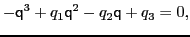
with two functions  and
and  of the two scalars and .
Eq. (54) is a direct consequence of the Cayley-Hamilton Theorem and thus
can be called the Cayley-Hamilton theorem for the quadrupole tensors. It can be generalized
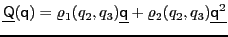
for the isotropic tensor field
of the two scalars and .
Eq. (54) is a direct consequence of the Cayley-Hamilton Theorem and thus
can be called the Cayley-Hamilton theorem for the quadrupole tensors. It can be generalized
for the isotropic tensor field
 with an arbitrary multipolarity
  being a function of one or a few spherical tensors
 ,
,
 of ranks
  ,
,
 , respectively.
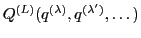
The Generalized Cayley-Hamilton Theorem has the following general form:
, respectively.
The Generalized Cayley-Hamilton Theorem has the following general form:
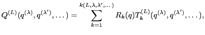 |
(55) |
where  stands for the set of independent scalars,
  are some definite fundamental tensors, all
constructed from
,
, and
are some definite fundamental tensors, all
constructed from
,
, and  are arbitrary scalar functions.
The number
are arbitrary scalar functions.
The number
 depends on the ranks of the all involved tensors. To find the number and the forms of
the fundamental tensors in a general case may appear to be a difficult task. A systematic
method of constructing them in the case of the tensor fields depending on one tensor are presented
in Refs.[6,8]
Eqs. (20)-(22) are examples of the GCH theorem
for
depends on the ranks of the all involved tensors. To find the number and the forms of
the fundamental tensors in a general case may appear to be a difficult task. A systematic
method of constructing them in the case of the tensor fields depending on one tensor are presented
in Refs.[6,8]
Eqs. (20)-(22) are examples of the GCH theorem
for
 and
and
 , whereas Eqs. (23)-(25) --
for
, whereas Eqs. (23)-(25) --
for
 and
. In the nuclear collective model the GCH theorem was used for
and
. In the nuclear collective model the GCH theorem was used for
 and
and
 .[14,15]
Next: Acknowledgements
Up: SPATIAL SYMMETRIES OF THE
Previous: Summary
Jacek Dobaczewski
2010-01-30