Transition matrix elements and transition densities

Calculation of the matrix elements in Eq. (15) between the original and shifted HFB states is straightforward, because the shifted states also belong to the family of the HFB states. In particular, their overlap is given by the Onishi formula [1], which in the canonical basis reduces to a simple expression,

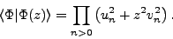$$\langle\Phi\vert\Phi(z)\rangle = \prod_{n>0}\left(u_n^2+ z^2 v_n^2\right) .$$ (25)

Similarly, the generalized Wick's theorem [1] can be used for evaluation of Hamiltonian matrix elements,

$$\langle\Phi\vert\hat{H}\vert\Phi(z)\rangle = \langle\Phi\ver... ..., E_{\mbox{\rm\scriptsize {HFB}}}(\rho_z,\chi_z,\bar{\chi}_z),$$ (26)

where the so-called HFB transition energy density $E_{\mbox{\rm\scriptsize {HFB}}}(\rho_z,\chi_z,\bar{\chi}_z)$ is a function of the shifted particle and pairing transition density matrices,

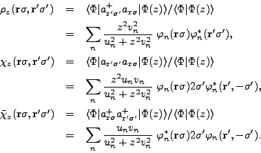$$\begin{array}{lll} \rho_z({\bf r}\sigma,{\bf r}'\sigma') &... ...{\bf r}\sigma)2\sigma'\varphi_n({\bf r}',-\sigma'). \end{array}$$ (27)

The transition density matrices become the standard density matrices in the limit of $z\rightarrow 1$. For simplicity, we do not explicitly show the isospin variables; this is not essential in the context of the present work. (See Ref. [13] for a complete formulation.)