


Next: Results
Up: Angular momentum projection of
Previous: Introduction
Methods
The angular-momentum-conserving wave function is obtained by employing
the standard operator
 [15,16] projecting
onto angular momentum
[15,16] projecting
onto angular momentum  , with projections
  and
and  along the
laboratory and intrinsic
along the
laboratory and intrinsic  axes, respectively,
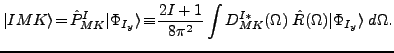 |
(2) |
Here,
 represents the set of three Euler angles
 ,
,
 are the Wigner
functions [17],
and
are the Wigner
functions [17],
and
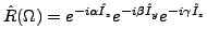 is the rotation operator.
Since is not a good quantum number, different components must
be mixed with the mixing coefficients determined by the minimization
of energy. The -mixing is realized in a standard way by assuming:
 |
(3) |
and by solving the following Hill-Wheeler (HW) [18] equation:
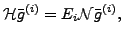 |
(4) |
where
 and
and
 denote the Hamiltonian and overlap kernels, respectively,
and
denote the Hamiltonian and overlap kernels, respectively,
and
 denotes a column of the
  coefficients.
The overlap and Hamiltonian kernels have their
standard functional form but depend upon transition (or mixed)
density matrices between rotated states:
coefficients.
The overlap and Hamiltonian kernels have their
standard functional form but depend upon transition (or mixed)
density matrices between rotated states:
 |
(5) |
The transition density matrix is also used for the
density-dependent term. This is the only prescription
available so far satisfying certain consistency criteria,
formulated and thoroughly discussed in Refs. [5,19].
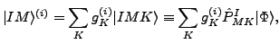
Due to the overcompleteness of the
 states, Eq. (4) is solved within the
so-called collective subspace spanned by the natural
states:
states, Eq. (4) is solved within the
so-called collective subspace spanned by the natural
states:
 |
(6) |
which are eigenstates of the norm matrix
 having
non-zero eigenvalues (
having
non-zero eigenvalues ( ):
):
 |
(7) |
In practical applications, the cutoff parameter  is
used and the collective subspace is constructed by using only those natural
states that satisfy
is
used and the collective subspace is constructed by using only those natural
states that satisfy
 . By ordering indices
  of the natural states
in such a way that larger indices correspond to smaller norm eigenvalues,
we can write the solutions of the HW equation (4) as:
of the natural states
in such a way that larger indices correspond to smaller norm eigenvalues,
we can write the solutions of the HW equation (4) as:
 |
(8) |
where the mixing coefficients of Eq. (3) read:
 |
(9) |
We can now define two types of the -mixing. On the one hand,
by the kinematic -mixing
we understand the situation where only one collective state is used,
i.e.,
 . Then, the solution of the HW equation
amounts to calculating only one matrix element of the Hamiltonian kernel,
. Then, the solution of the HW equation
amounts to calculating only one matrix element of the Hamiltonian kernel,
 |
(10) |
i.e.,
 and
and
 for
for  . In the kinematic
-mixing, the mixing coefficients
. In the kinematic
-mixing, the mixing coefficients
 are entirely determined by the norm kernel
and do not depend on the Hamiltonian kernel, i.e., they are entirely
given by the cranking approximation and Coriolis coupling. On the
other hand, by the dynamic -mixing we understand the full solution
of the HW equation for
are entirely determined by the norm kernel
and do not depend on the Hamiltonian kernel, i.e., they are entirely
given by the cranking approximation and Coriolis coupling. On the
other hand, by the dynamic -mixing we understand the full solution
of the HW equation for
 , where the cutoff
parameter is adjusted so as to obtain a plateau condition for
the lowest eigenvalue
, where the cutoff
parameter is adjusted so as to obtain a plateau condition for
the lowest eigenvalue  . Here, the generator-coordinate-method (GCM)
mixing of different
components becomes effective, which potentially can modify the
cranking mixing coefficients. We stress here that the kinematic
-mixing does correspond to a -mixed solution too, and is not
assuming any single given value of .
. Here, the generator-coordinate-method (GCM)
mixing of different
components becomes effective, which potentially can modify the
cranking mixing coefficients. We stress here that the kinematic
-mixing does correspond to a -mixed solution too, and is not
assuming any single given value of .
The deformed CHF states were provided by the code HFODD, which solves
the Hartree-Fock equations that correspond to the Ritz variational
principle,
 |
(11) |
with angular frequency  adjusted so as to fulfill constraint
(1) and the value of
adjusted so as to fulfill constraint
(1) and the value of  being equal to , according to our
 scheme. The
  -signature and parity symmetries
were conserved.
The Hamiltonian and overlap kernels were calculated using the
Gauss-Chebyshev quadrature in the
-signature and parity symmetries
were conserved.
The Hamiltonian and overlap kernels were calculated using the
Gauss-Chebyshev quadrature in the  and
and  directions
and the Gauss-Legendre quadrature in the
directions
and the Gauss-Legendre quadrature in the  direction
[20]. In the numerical applications presented in this work
we used the SLy4 [21] Skyrme force, but similar results
were also obtained by using the SIII [22] force.
The time-odd terms in the Skyrme functional were fixed by using
values of the Landau parameters [23,24].
The harmonic-oscillator
basis was composed of 10 spherical shells. The
integration over the Euler angles was done by using a cube of
50
direction
[20]. In the numerical applications presented in this work
we used the SLy4 [21] Skyrme force, but similar results
were also obtained by using the SIII [22] force.
The time-odd terms in the Skyrme functional were fixed by using
values of the Landau parameters [23,24].
The harmonic-oscillator
basis was composed of 10 spherical shells. The
integration over the Euler angles was done by using a cube of
50 5050 integration points.
Next: Results
Up: Angular momentum projection of
Previous: Introduction
Jacek Dobaczewski
2007-08-08