Next: The direct part of
Up: Results
Previous: The Lipkin method
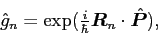
The Lipkin operator
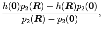
A practical method to calculate the correcting constant  from
Eq. (18) must not involve, of course, the exact evaluation of
the function
from
Eq. (18) must not involve, of course, the exact evaluation of
the function
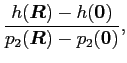
 . A method to probe the function
without evaluating it explicitly can be formulated
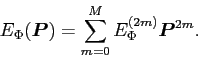
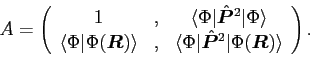
as follows. One first remarks that the projected energy (4)
can also be calculated as:
. A method to probe the function
without evaluating it explicitly can be formulated
as follows. One first remarks that the projected energy (4)
can also be calculated as:
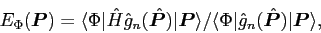 |
(20) |
which gives the sum rules:
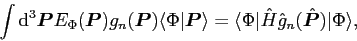 |
(21) |
where
 are arbitrary functions of
  .
By using different functions
.
By using different functions  , one can probe the
unknown function
.
, one can probe the
unknown function
.
An obvious choice of
 , which, in
fact, has been used within the Lipkin-Nogami method [7] to
restore the particle number, requires dealing with impractical
many-body operators. A much better option is provided by the shift
operators [cf. Eq. (1) and (2)],
, which, in
fact, has been used within the Lipkin-Nogami method [7] to
restore the particle number, requires dealing with impractical
many-body operators. A much better option is provided by the shift
operators [cf. Eq. (1) and (2)],
 |
(22) |
defined for a suitably selected values of shifts  . Then,
the average values on the right-hand side of Eq. (21) become
equal to the energy kernels
. Then,
the average values on the right-hand side of Eq. (21) become
equal to the energy kernels  , which are very easy to
calculate.
, which are very easy to
calculate.
In practice, the method works as follows. Suppose one wants to evaluate
the Taylor-expansion coefficients of
up to a given order of  ,
,
 |
(23) |
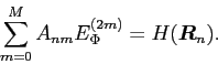
After inserting this into Eq. (21), one obtains the
set of linear equations,
 |
(24) |
where the matrix  is defined by the kernels of the momentum operators:
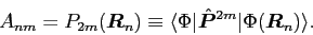 |
(25) |
In the simplest case of the quadratic Lipkin operator, Eq. (14),
one only needs the expansion up the second order, that is, for  .
Then, by using two points
.
Then, by using two points
 and
and
 one obtains
 |
(26) |
This matrix can be easily inverted and then one obtains the first
two Taylor expansion coefficients  and
and  ,
which are required in Eq. (18), that is,
,
which are required in Eq. (18), that is,
where the reduced kernel of the momentum operator is defined as
usually, by
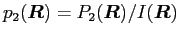 . Expressions
(27) and (28) can be very easily evaluated,
especially in view of the fact that the momentum kernel can
be calculated as a Laplacian of the overlap kernel:
. Expressions
(27) and (28) can be very easily evaluated,
especially in view of the fact that the momentum kernel can
be calculated as a Laplacian of the overlap kernel:
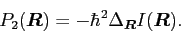 |
(29) |
Of course, within the GOA, the results are exactly the same as
those given by the zero-point-motion correction and PY
mass, Eqs. (10) and (11). However, expressions
(27) and (28) do not rely on the GOA.
They only depend on assuming the quadratic form of the Lipkin
operator  , Eq. (14). Moreover, variations of explicit
expressions for the projected energy
, Eq. (14). Moreover, variations of explicit
expressions for the projected energy
 , like the ones
given by Eqs. (9) or (27), are difficult, while that
of the Lipkin projected energy (19) can be carried out by
the standard self-consistent procedure.
, like the ones
given by Eqs. (9) or (27), are difficult, while that
of the Lipkin projected energy (19) can be carried out by
the standard self-consistent procedure.
When the quadratic
approximation is not sufficient, one can immediately notice this fact
by a dependence of
and on the value of the shift
 . In this case, one can always switch to higher-order
Lipkin operators:
. In this case, one can always switch to higher-order
Lipkin operators:
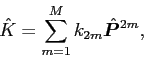 |
(30) |
which would require using higher-order Taylor expansions
(23), and  different shifts ,
 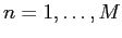 ,
instead of one. The only requirement for choosing the shifts
is a non-singularity of the matrix
,
instead of one. The only requirement for choosing the shifts
is a non-singularity of the matrix  . A dependence of
the results on this choice will always give a signal that a given
order is insufficient. Note that kernels of higher powers of the
momentum operator can also be calculated in terms of higher
derivatives of the overlap kernel, in analogy with Eq. (29).
However, in view of the fact that for the translational symmetry the
GOA works so nicely, in this study there does not seem to be any
immediate necessity to go to higher orders, and the simple quadratic
correction will suffice.
. A dependence of
the results on this choice will always give a signal that a given
order is insufficient. Note that kernels of higher powers of the
momentum operator can also be calculated in terms of higher
derivatives of the overlap kernel, in analogy with Eq. (29).
However, in view of the fact that for the translational symmetry the
GOA works so nicely, in this study there does not seem to be any
immediate necessity to go to higher orders, and the simple quadratic
correction will suffice.
Figure 5:
(Color online) The Lipkin projected energies (19)
calculated in 9 doubly-magic spherical nuclei, and plotted relative to
the standard energies calculated for the SLy4 Skyrme functional
[9]. Open and full squares show results obtained
for the exact [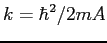 ] and calculated
[Eq. (28)] correcting factors, respectively. Solid
line shows the fit of the volume and surface terms.
] and calculated
[Eq. (28)] correcting factors, respectively. Solid
line shows the fit of the volume and surface terms.
![\includegraphics[angle=0,width=0.7\columnwidth]{renmas.fig5.eps}](img99.png) |
Figure 6:
(Color online) Exact masses ( , open squares) and the PY masses
calculated after the Lipkin minimization from
Eq. (28) (
, open squares) and the PY masses
calculated after the Lipkin minimization from
Eq. (28) ( , full squares), compared
with the PY masses of Fig. 4 (full circles).
, full squares), compared
with the PY masses of Fig. 4 (full circles).
![\includegraphics[angle=0,width=0.7\columnwidth]{renmas.fig6.eps}](img102.png) |
Next: The direct part of
Up: Results
Previous: The Lipkin method
Jacek Dobaczewski
2009-06-28