Introduction

Self-consistent mean-field method is practically the only formalism allowing for large-scale computations in heavy, open-shell nuclei with many valence particles. Inherent to the mean-field method is a mechanism of the spontaneous symmetry breaking, which is essentially the only way allowing to incorporate a significant part of many-body correlations into a single intrinsic (symmetry-violating) Slater determinant. Nuclear deformation and the emergence of rotational bands after applying simple cranked mean-field approach, i.e., after an approximate restoration of rotational invariance, is one of the most spectacular and most intuitive manifestations of the spontaneous symmetry breaking in nuclei.

An increasing quality of spectroscopic information demands more and more accurate theory, pushing the efforts beyond the mean-field approximation towards, in particular, symmetry-conserving formalisms and symmetry restoration.[1,2,3] Hereby, we report on development of a new theoretical tool allowing for the angular-momentum projection (AMP) of cranked symmetry-unrestricted Slater determinants.

The standard method used to develop symmetry-conserving theory, starting from intrinsic (deformed) wave function $\vert\Phi\rangle$, obtained within the mean-field approach, is provided by the projection techniques onto eigenspaces of symmetry operators. There are two practical realizations of the projection methods: more fundamental and elaborate variation after projection (VAP) and slightly less advanced projection after variation (PAV). In the past, many calculations have been performed within the angular-momentum PAV method, where non-rotating states have been projected, see, e.g., Refs.[4,5,6] and the reviews in Refs.[2,3]. The cranking method provides the first-order approximation to the angular-momentum VAP method.[1] However, after the ground-breaking studies in Refs.[7,8], calculations based on the AMP of cranked states have not been performed. Here, we present the first results of our recently developed AMP method of cranked symmetry-unrestricted Hartree-Fock states. The procedure we use has been implemented within the code HFODD (v2.25b).[9,10,11,12]

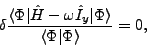
We determine the optimal product wave function $\vert\Phi\rangle$ by using the cranked self-consistent Skyrme-Hartree-Fock (SHF) method. The Ritz variational principle:

$$\delta \frac{\langle \Phi \vert\hat H-\omega\hat{I}_y\vert \Phi \rangle}{\langle \Phi\vert\Phi \rangle} = 0,$$ (1)

is equivalent to a variation of a local energy density functional (LEDF) with a supplementary constraint on the average value of the projection of angular momentum on the axis perpendicular to the symmetry axis ($y$ in our case). The variation of LEDF in the isoscalar-isovector $t=0,1$ representation (potential part) can be formally written as:

$$\delta \mathcal{E}^{(Skyrme)}= \delta \sum_{t=0,1}\int d^3\ma... ...{H}_t^{(TE)}(\mathbf{r}) + \mathcal{H}_t^{(TO)}(\mathbf{r}) ].$$ (2)

where $\mathcal{H}_t(\mathbf{r})$ is expressed as a bilinear form of the time-even (TE) $\rho, \tau, J$ and time-odd (TO) $\mathbf{s}$, $\mathbf{T}$, $\mathbf{j}$ local densities and currents, and by their derivatives,[13]

$$\mathcal{H}_t^{(TE)}(\mathbf{r}) = C^{\rho}_t \rho^2_t + C^{... ...t + C^{\nabla J}_t \rho_t \mathbf{\nabla } \cdot \mathbf{J}_t,$$ (3)

$$\mathcal{H}_t^{(TO)}(\mathbf{r}) = C^{s}_t \mathbf{s}^2_t + ... ...j}_t \mathbf{s}_t \cdot (\mathbf{\nabla} \times \mathbf{j}_t).$$ (4)

By taking an expectation value of the Skyrme force over the Slater determinant, one obtains the LEDF (3)-(4) with $20$ coupling constants $C$ that are expressed uniquely through the 10 parameters $x_i, t_i, i = 0, 1, 2, 3,$ and $W, \alpha$ of the standard Skyrme force. Because of the local gauge invariance of the Skyrme force, only 14 coupling constants $C$ are independent quantities. The local gauge invariance links three pairs of time-even and time-odd constants in the following way:

$$C^j_t = - C^{\tau}_t, \quad \quad C^J_t = - C^T_t, \quad \quad C^{\nabla j}_t = C^{\nabla J}_t.$$ (5)