


Next: Conclusions
Up: ANGULAR-MOMENTUM PROJECTION OF CRANKED
Previous: Angular-Momentum Projection
Figure 1:
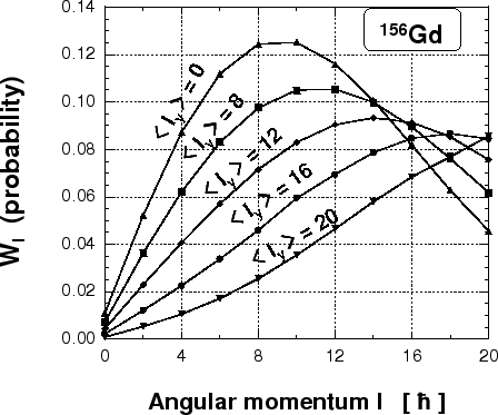
Probability distributions of even angular-momentum
components  in
in  Gd.
Gd.
 |
We solve the cranked SHF equations for Gd by using
the code HFODD for
the SIII Skyrme-force parameters[16] and spherical harmonic-oscillator
basis composed of  =10 shells.
Then, we calculate the Hamiltonian and overlap kernels by using
50 Gauss-Chebyshev integration points in the
=10 shells.
Then, we calculate the Hamiltonian and overlap kernels by using
50 Gauss-Chebyshev integration points in the  and
and  directions and 50 Gauss-Legendre points in the
  direction.[12]
Figure 1 shows probability distributions
direction.[12]
Figure 1 shows probability distributions  of even angular-momentum components
in the intrinsic cranked-SHF states
of even angular-momentum components
in the intrinsic cranked-SHF states
 constrained to
 . The probability of finding the component can be
calculated from:[1]
. The probability of finding the component can be
calculated from:[1]
 |
(10) |
The curves correspond to cranking wave functions with
averaged angular momenta
 , and
, and
 . One can see that for low angular momenta (e.g., for
 ) the maxima of the distributions do not lie near the same
values of
) the maxima of the distributions do not lie near the same
values of
 . Similar results have been
obtained by Islam et al.[7] and Baye et
al.[8].
. Similar results have been
obtained by Islam et al.[7] and Baye et
al.[8].
Figure 2:
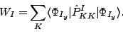
Probability distributions of projections  in
the even angular-momentum components projected from the state with
in
the even angular-momentum components projected from the state with
 in Gd.
 |
In Fig. 2 we show similar probability distributions  of
the projections ,
of
the projections ,
 |
(11) |
projected from the state with
in Gd.
One can see that the  component dominates for all angular
momenta, while the
component dominates for all angular
momenta, while the  components increase with the increasing
angular momentum. The
components increase with the increasing
angular momentum. The  component is the second in magnitude
after , which illustrates the build-up of the Coriolis coupling in
a rotating intrinsic state. Note that only even values of can
be projected from the non-rotating
component is the second in magnitude
after , which illustrates the build-up of the Coriolis coupling in
a rotating intrinsic state. Note that only even values of can
be projected from the non-rotating
 state,
while all
state,
while all  appear in the cranked state.
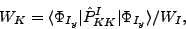
In order to find energies of the AMP states, we solve Eq. (9)
by diagonalizing first the norm matrix:
 |
(12) |
The non-zero eigenvalues ( ) of
) of  are used afterwards to
built the so-called natural states
are used afterwards to
built the so-called natural states
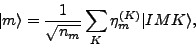 |
(13) |
that span the subspace called collective subspace. Final diagonalization
of the HW equation (9) is performed within the collective subspace.
In this subspace the problem reduces
to the standard hermitian eigenvalue problem.
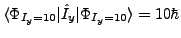
Figure 3:
Dependence of energies of projected states on the number of
the norm eigenstates kept in the collective subspace. Angular momenta
 were projected from the state having the average
projection of angular momentum
were projected from the state having the average
projection of angular momentum
 .
.
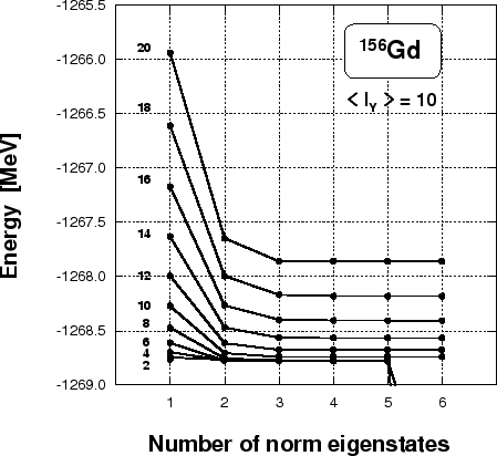 |
In practical numerical applications we use the cut-off parameter
 to construct the collective subspace, by keeping only the
norm eigenstates (12) with
to construct the collective subspace, by keeping only the
norm eigenstates (12) with  . The test depicted
in Fig. 3 shows the stability of projected solutions with
respect to the number of the norm eigenstates kept in the collective
subspace. The analysis was conducted for angular-momentum
states projected from the deformed solution
. The test depicted
in Fig. 3 shows the stability of projected solutions with
respect to the number of the norm eigenstates kept in the collective
subspace. The analysis was conducted for angular-momentum
states projected from the deformed solution
 obtained by solving the cranked SHF equations
with the constraint
obtained by solving the cranked SHF equations
with the constraint
 . The test clearly shows that,
starting from a certain point, the obtained solutions are stable
(plateau condition). Only for very small values of
. The test clearly shows that,
starting from a certain point, the obtained solutions are stable
(plateau condition). Only for very small values of
 the method becomes numerically unstable.
Figure 4:
Rotational bands in Gd nucleus:
the four bands represent:
(a) experimental data,
(b) cranked SHF calculations,
(c) band projected from the state
 , and
(d) band projected from the state
, and
(d) band projected from the state
 into ,
for
into ,
for
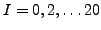 .
.
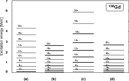 |
Figure 4 shows rotational bands (b)-(d) calculated in
Gd in comparison with the experimental data (a). Band (b)
represents the average mean-field energies obtained from the cranked
SHF calculations by constraining solutions to
 .
In bands (c) and (d), we show energies obtained by the AMP from the
and
, respectively. We
see, that band (c) is much higher than bands (b) and (d), which
indicates that the PAV from the
state is not
an adequate method of describing nuclear rotation. Note that the
mean-field energies (b) and the AMP energies (d) corresponding to
turn out to be very similar to one another.
This shows that the AMP from the
states
constitutes a correct symmetry restoration of the approximate VAP
solutions realized by the cranking procedure. The remaining
discrepancy with experimental data must be attributed to pairing
correlations, which are not included in our SHF solutions.
.
In bands (c) and (d), we show energies obtained by the AMP from the
and
, respectively. We
see, that band (c) is much higher than bands (b) and (d), which
indicates that the PAV from the
state is not
an adequate method of describing nuclear rotation. Note that the
mean-field energies (b) and the AMP energies (d) corresponding to
turn out to be very similar to one another.
This shows that the AMP from the
states
constitutes a correct symmetry restoration of the approximate VAP
solutions realized by the cranking procedure. The remaining
discrepancy with experimental data must be attributed to pairing
correlations, which are not included in our SHF solutions.
When calculating the Hamiltonian kernels within the LEDF approach,
one has to use transition density matrices between rotated states,
 |
(14) |
which are singular whenever the rotated states are orthogonal.
In particular, the transition multipole moments,
 |
(15) |
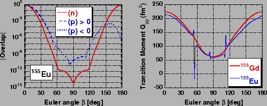
become singular for certain values of the Euler angles  . This
is illustrated in Fig. 5, which shows absolute values of
the neutron and proton overlap kernels in
. This
is illustrated in Fig. 5, which shows absolute values of
the neutron and proton overlap kernels in  Eu (left panel), and
the transition quadrupole moments
Eu (left panel), and
the transition quadrupole moments
 in Eu and
Gd (right panel). Calculations have been performed for axial
shapes of nuclei, for which only the rotation about the Euler angle
matters. The neutron overlap kernel corresponds to an even
number of particles (
in Eu and
Gd (right panel). Calculations have been performed for axial
shapes of nuclei, for which only the rotation about the Euler angle
matters. The neutron overlap kernel corresponds to an even
number of particles ( ), and is always positive, although at
 it becomes as small as
  . On the other
hand, the proton overlap kernel corresponds to an odd number of
particles (
. On the other
hand, the proton overlap kernel corresponds to an odd number of
particles ( ), and it three times changes the sign in the
interval of
), and it three times changes the sign in the
interval of
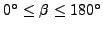 . Consequently, the
transition quadrupole moment of Gd is a regular function,
while that of Eu has three poles.
. Consequently, the
transition quadrupole moment of Gd is a regular function,
while that of Eu has three poles.
Figure 5:
Left panel: Dependence of the absolute value of the overlap
between rotated states on the Euler angle in Eu.
Solid line shows the neutron overlap that is always positive.
Dashed and dotted lines show these segments of the proton overlap where it is
positive and negative, respectively.
Right panel: Transition quadrupole moments  versus in Gd
(thick line) and Eu (thin line).
versus in Gd
(thick line) and Eu (thin line).
 |
Of course, when calculating the matrix elements of multipole
operators between the rotated states, the transition matrix elements
(15) are multiplied by the overlap kernels and the poles
disappear. However, such a compensation is absent for kernels
corresponding to higher powers of densities, viz. for the
density-dependent terms of the Skyrme interactions, or for the
direct-Coulomb-energy terms, or for the exchange-Coulomb-energy terms
in the Slater approximation. How to treat such singular kernels
within the AMP methods is currently an open and unsolved problem,
similarly as is the case for the particle-number-projection methods
recently discussed in Ref.[17].
Next: Conclusions
Up: ANGULAR-MOMENTUM PROJECTION OF CRANKED
Previous: Angular-Momentum Projection
Jacek Dobaczewski
2006-10-30