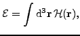
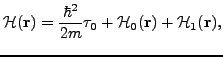
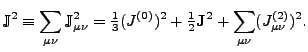
We begin by recalling the form of the EDF, which will be used in the present study. In the notation defined in Ref. [10] (see Ref. [11] for more details and extensions), the EDF reads
In particular, the SO density
![]() is the vector part of the spin-current tensor density
is the vector part of the spin-current tensor density
![]() , i.e.,
, i.e.,
In the context of the present study, the time-even tensor and SO parts of the EDF,
In the spherical-symmetry limit, the scalar ![]() and symmetric-tensor
and symmetric-tensor
![]() parts of the spin-current tensor vanish,
and thus
parts of the spin-current tensor vanish,
and thus
Identical potential-energy terms of the EDF, Eqs. (4) and (5),
are obtained by averaging the
Skyrme effective interaction within the Skyrme-Hartree-Fock (SHF)
approximation [3]. By this procedure, the EDF coupling
constants ![]() can be expressed through the Skyrme-force parameters,
and one can use parameterizations existing in the literature. It is
clear that one can study tensor and SO effects entirely within the
EDF formalism, i.e., by considering the corresponding tensor and SO
parts of the EDF, Eqs. (8) and (9), and coupling constants
can be expressed through the Skyrme-force parameters,
and one can use parameterizations existing in the literature. It is
clear that one can study tensor and SO effects entirely within the
EDF formalism, i.e., by considering the corresponding tensor and SO
parts of the EDF, Eqs. (8) and (9), and coupling constants
![]() and
and
![]() , respectively. However, in order to link this approach
to those based on the Skyrme interactions, we recall here expressions
based on averaging the zero-range tensor and SO forces [13,14], see
also Refs. [11,15,16] for recent
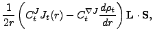
analyses. Namely, in the spherical-symmetry limit, one has
, respectively. However, in order to link this approach
to those based on the Skyrme interactions, we recall here expressions
based on averaging the zero-range tensor and SO forces [13,14], see
also Refs. [11,15,16] for recent
analyses. Namely, in the spherical-symmetry limit, one has
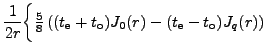
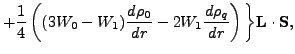
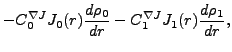
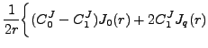
The corresponding SO MFs read
In this exploratory work, we base our considerations on the EDF
method and deliberately break the connection between the functional
(4), and the Skyrme central, tensor, and SO forces.
Nevertheless, in the time-even sector, our starting point is the
conventional Skyrme-force-inspired functional with coupling constants fixed
at the values characteristic for either
SkP [18], SLy4 [19], or SkO [20]
Skyrme parameterizations. However, poorly known coupling constants in
the time-odd sector (those which are not related to the time-even ones
through the local-gauge invariance [10]) are fixed
independently of their Skyrme-force values. For this purpose, the
spin coupling constants ![]() are readjusted to reproduce
empirical values of the Landau parameters, according to the
prescription given in Refs. [21,22], and
are readjusted to reproduce
empirical values of the Landau parameters, according to the
prescription given in Refs. [21,22], and
![]() are set equal to zero. These variants of the standard
functionals are below denoted by SkP
are set equal to zero. These variants of the standard
functionals are below denoted by SkP![]() , SLy4
, SLy4![]() , and SkO
, and SkO![]() .
.
Strictly pragmatic reasons, like technical complexity and lack of
firm experimental benchmarks, made the majority of older Skyrme
parameterizations simply disregard the tensor terms, by setting
![]() . However, suggestions to study tensor effects
on a one-body level were already made long time ago
[13,14,23,24].
Recent experimental discoveries of new magic
shell-openings in neutron-reach light nuclei, e.g., around
. However, suggestions to study tensor effects
on a one-body level were already made long time ago
[13,14,23,24].
Recent experimental discoveries of new magic
shell-openings in neutron-reach light nuclei, e.g., around ![]() [25,26], and their subsequent interpretation in terms
of tensor interaction within the
shell-model [27,28,29], caused a revival of
interest in tensor terms within the MF approach
[30,15,31,32,34,35,33,16,,37,38],
which is
naturally tailored to study s.p. levels. Indeed, as shown in
Ref. [15], the tensor terms mark clear and unique
fingerprints in isotonic and isotopic evolution of s.p. levels and,
in particular, in the SO splittings.
[25,26], and their subsequent interpretation in terms
of tensor interaction within the
shell-model [27,28,29], caused a revival of
interest in tensor terms within the MF approach
[30,15,31,32,34,35,33,16,,37,38],
which is
naturally tailored to study s.p. levels. Indeed, as shown in
Ref. [15], the tensor terms mark clear and unique
fingerprints in isotonic and isotopic evolution of s.p. levels and,
in particular, in the SO splittings.
Below we consider one example of the Skyrme force (SkP), which does
contain the usual ![]() terms in the energy functional, and two
examples of forces (SLy4 and SkO) that set these terms equal to zero.
For the latter forces, there exist also variants (SLy5 and SkO') that
do include the
terms in the energy functional, and two
examples of forces (SLy4 and SkO) that set these terms equal to zero.
For the latter forces, there exist also variants (SLy5 and SkO') that
do include the ![]() terms. We have checked that conclusions of our
study do not depend on which of these variants are considered.
terms. We have checked that conclusions of our
study do not depend on which of these variants are considered.
In this paper, we perform systematic study of the SO splittings. The
goal is to resolve contributions to the SO MF (12) due
to the tensor and SO parts of the EDF, and to readjust the
corresponding coupling constants ![]() and
and
![]() . It is
shown that this goal can be essentially achieved by studying the
. It is
shown that this goal can be essentially achieved by studying the
![]() SO splittings in three key nuclei:
SO splittings in three key nuclei: ![]() Ca,
Ca,
![]() Ca, and
Ca, and ![]() Ni. Before we present in Sec. 4 details
of the fitting procedure and values of the obtained coupling
constants, first we discuss effects of the core polarization and its
influence on the calculated and SO splittings.
Ni. Before we present in Sec. 4 details
of the fitting procedure and values of the obtained coupling
constants, first we discuss effects of the core polarization and its
influence on the calculated and SO splittings.
![$\displaystyle {\mathcal H}_{SO} = \frac{1}{4}\left[3W_0J_0(r)\frac{d\rho_0}{dr} +W_1J_1(r)\frac{d\rho_1}{dr}\right],$](img51.png)