The Quasiparticle Formalism

We begin by recalling basic equations of the quasiparticle formalism, which historically is attributed to Gor'kov, Bogoliubov, and de Gennes. While these equations and definitions are admittedly very well known, there are several aspects of the quasiparticle approach that are seldom discussed; hence, they are worth bringing to the attention of a wider community. We shall discuss these lesser-known aspects in the subsections following the general introduction to HFB.

The HFB wave functions are quasiparticle product states. The quasiparticle annihilation operators $\alpha_\mu$ are defined as linear combinations of particle annihilation and creation operators by the Bogoliubov transformation,

$$\alpha_\mu := \sum_\nu \left(U^*_{\nu\mu} a_\nu + V^*_{\nu\mu}a^+_\nu \right).$$ (1)

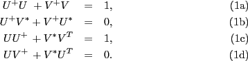
The matrices $U$ and $V$ satisfy the following canonical conditions: The HFB vacuum $\vert\Psi\rangle$ is a zero-quasiparticle state:

$$\alpha_\mu\vert\Psi\rangle=0.$$ (2)

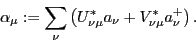
Complete information about $\vert\Psi\rangle$ is, in fact, contained in the generalized density matrix ${\mathcal{R}}$,

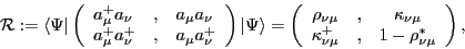$$\mathcal{R} := \langle\Psi\vert\left(\begin{array}{lcl}{a^+... ... \kappa^+_{\nu\mu} &,& 1-\rho^*_{\nu\mu} \end{array}\right),$$ (3)

which in terms of matrices $U$ and $V$ reads:

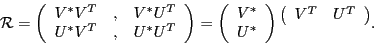$$\mathcal{R} = \left(\begin{array}{ccc} V^*V^T &,& V^*U^T \\... ...m}{$ \left(\begin{array}{cc} V^T & U^T \end{array}\right)$} .$$ (4)

The variational principle implies that the self-consistent density matrix ${\mathcal{R}}$ commutes with the quasiparticle Hamiltonian

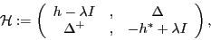$$\mathcal{H} := \left(\begin{array}{ccc} h-\lambda I &,& \Delta \\ \Delta^+&,& -h^*+\lambda I\end{array}\right) ,$$ (5)

where $h=t+\Gamma$ is the single-particle Hamiltonian and $\Gamma$ and $\Delta$ are particle-hole and particle-particle mean-fields, respectively. The HFB equations can be written in a matrix form:

$$\left(\begin{array}{ccc} h-\lambda I &,& \Delta \\ \Delta... ...(\begin{array}{ccc} E &,& 0 \\ 0 &,& -E \end{array}\right) ,$$ (6)

where $E$ is a diagonal matrix of quasiparticle energies $E_\mu$. Columns of eigenvectors,

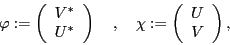$$\varphi := \left(\begin{array}{c} V^* \\ U^* \end{array}\ri... ...uad \chi := \left(\begin{array}{c} U \\ V \end{array}\right),$$ (7)

are called occupied and empty quasiparticle states, respectively, because they are eigenvectors of the projective matrix $\mathcal{R}$ with eigenvalues 1 and 0.