Atomic and nuclear HFB calculations

The first numerical example of 2FLA deals with a two-component polarized atomic condensate in a deformed harmonic trap using the superfluid local density approximation [34,10]. The system is described by a local energy density

$$\mathcal{E}(\boldsymbol{r}) = \alpha_{u}\frac{\tau(\boldsy... ... g_{eff}(\boldsymbol{r}) \vert{\kappa}(\boldsymbol{r})\vert^2,$$ (30)

where the local densities $\rho(\boldsymbol{r})$ (particle density), $\tau(\boldsymbol{r})$ (kinetic energy density), and $\kappa(\boldsymbol{r})$ (pairing tensor) are constructed from the quasiparticle HFB wave functions. The parameters $\alpha_u$, $\beta_u$, and the effective pairing strength $g_{eff}(\boldsymbol{r})$ have been taken according to Ref. [10]. We assume that the external trapping potential can be described by an axially deformed harmonic oscillator with frequencies [17]

$$\omega_\perp^2(\delta)=\omega_0^2(\delta)\left(1+{2\over 3}\... ...x^2(\delta)=\omega_0^2(\delta)\left(1-{4\over 3}\delta\right),$$ (31)

with

$$\omega_0(\delta)=\tilde{\omega}_0\left(1+{2\over 3}\delta^2\right).$$ (32)

As in Ref. [10], we put $\hbar\tilde{\omega}_0$=1.

The calculations were carried out for systems with $N$=30 and 31 fermions in a spherical ($\delta$=0) and deformed ($\delta$=0.2) trap. The HFB equations were solved by using the recently developed axial DFT solver HFB-AX [35]. The results are displayed in Fig. 3.

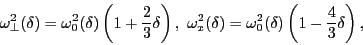
Figure 3: (Color online) Quasiparticle levels ($\alpha$=1/2: solid line; $\alpha$=-1/2: dotted line) as functions of $\lambda _s$ for a two-component polarized atomic condensate in a deformed harmonic trap using the superfluid local density approximation [34,10]. The calculations were carried out for $N$=30 (left) and $N$=31 (right). The top panels correspond to the spherical case ($\delta$=0). Here the quasiparticle levels are labeled with the usual spectroscopic designation of orbital angular momentum $\ell$. Each line represents a set of (2$\ell$+1)-fold degenerate states. In the deformed case ($\delta$=0.2; middle panels) the levels with the opposite values of $\Lambda$$>$0 are two-fold degenerate. The corresponding values of $\vert\Lambda \vert$ ere shown in the inset. The Kramers degeneracy can be lifted by adding a cranking term, $-\omega_\Lambda \hat{\ell}_x$ to the Hamiltonian (bottom panels, $-\omega _\Lambda$=0.05). Here, every level is labeled by the $\Lambda$ quantum number, see the inset. In order to make the plot less busy, the quasiparticle levels originating from very excited spherical $g$, $d$, and $s$ shells are not shown in the two lower panels. See text for details.

In the spherical case, Fig.3 (top), the spin degeneracy is lifted by the polarizing field $h_s$. However, as discussed in Sec. 3.2, the orbital $(2\ell$+1)-fold degeneracy is present. Consequently, after the crossing point, the vacuum becomes a $(2\ell_1$+1)-quasiparticle state, where $\ell_1$ is the orbital angular momentum of the lowest quasiparticle level. For $N$=30, the lowest quasiparticle excitation is a $p$ state, i.e., above the crossing point the local HFB vacuum becomes a three-quaspiarticle state. At the crossing point, the self-consistent mean-field changes abruptly. In particular, the chemical potential moves up as the number of particles increases by one, and the pairing gap decreases due to blocking. This produces a sharp discontinuity around the crossing point, which can be seen in all three cases presented in Fig. 3.

The middle portion of Fig. 3 illustrates the deformed case. Here, quasiparticle states are labeled using the angular momentum projection quantum number $\Lambda$ onto the symmetry axis of the trapping potential ($x$-axis). Because of the Kramers degeneracy, levels with $\pm\Lambda$ are degenerate. That is, except for $\Lambda$=0, each quasiparticle state is two-fold degenerate. In the case presented in Fig. 3, the two lowest levels have $\Lambda$=0, hence they are associated with one-quasiparticle excitations. The third state has $\vert\Lambda \vert$=1, and its crossing does not change the particle-number parity of the HFB vacuum.

The two-fold Kramers degeneracy can be removed by adding an external orbital-polarizing field,

$$\hat{h}_\ell=-\omega_\Lambda \hat{\ell}_x,$$ (33)

where $\omega_\Lambda$ is the cranking frequency for the orbital motion. Indeed, in the absence of the spin-orbit coupling the spin and the orbital angular momentum may rotate with different angular velocities. In the presence of the field (36), each level is shifted by $-\omega_\Lambda \Lambda$, i.e., the energy splitting of the Kramers doublet becomes $2\omega_\Lambda \vert\Lambda\vert$. An illustrative example of such situation is displayed in the bottom panels of Fig. 3. Here, each level corresponds to a one-quasiparticle excitation. We confirmed numerically that the result of calculations for $N$=31 by explicitly blocking the lowest level are here equivalent to those with 2FLA carried out above the crossing. It is seen in Fig. 3, however, that because of high density of quasiparticle levels, the self-consistent calculations in 2FLA are difficult due to many consecutive crossings that make it extremely difficult to keep track of the fixed configuration. We note that the order of the quasiparticle levels in $N$=30 and $N$=31 systems is affected by the variation of the mean field due to the crossing.

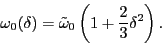
In order to illustrate 2FLA in the nuclear case, we carried out nuclear DFT calculations using the Skyrme energy density functional SLy4 [36] in the p-h channel, augmented by the ``mixed-pairing" [37] density-dependent delta functional in the p-p channel. The details pertaining to the numerical details, e.g. the pairing space employed, can be found in Ref. [35]. As a representative example, we took the pair of deformed nuclei $^{166}$Er ($N$=98) and $^{167}$Er ($N$=99). The pairing strength $V_0$=-320 MeVfm$^3$ was slightly enlarged to prevent pairing from collapsing in the $N$=99 system. The resulting neutron pairing gaps, $\Delta_n$=1.2MeV and 0.77MeV in $^{166}$Er and $^{167}$Er, respectively, are reasonably close to the experimental values of 1.02MeV and 0.62MeV.

Figure 4 displays the quasiparticle spectrum for $^{166}$Er (top) and $^{167}$Er (bottom).

Figure 4: (Color online) One-quasiparticle levels of both signatures ($\alpha$=1/2: solid line; $\alpha$=-1/2: dotted line) as functions of $\lambda _s$ for $^{166}$Er (top) and $^{167}$Er (bottom). The levels occupied in the vacuum configuration are drawn by thick lines. The calculations were carried out with a SLy4 Skyrme functional and mixed pairing. See text for details.

At the value of $\lambda _s$ indicated by a star symbol, a transition from a zero-quasiparticle vacuum corresponding to $N$=98 to a one-quasiparticle vacuum associated with $N$=99 takes place. As in the atomic case, the mean-field changes abruptly at the crossing point. Actually, since the quasiparticle spectrum changes when going from $^{166}$Er to $^{167}$Er (both in terms of excitation energy and ordering of levels), the crossing point is shifted towards the lower values of $\lambda _s$. As checked numerically, the result of calculations for $^{167}$Er by explicitly blocking the level ``a" are equivalent to those with 2FLA carried out above the crossing point.