

| Athens login |
|
|||
|
|
|
||
| IOP Journals Home | IOP Journals List | EJs Extra | This Journal | Search | Authors | Referees | Librarians | User Options | Help | | |||
| This volume |
|||
New J. Phys. 2 (2000)
19
PII: S1367-2630(00)13022-8
Error avoiding quantum codes and dynamical stabilization of Grover's algorithm
Michael Mussinger, Aldo Delgado and Gernot Alber
Abteilung für Quantenphysik, Universität Ulm, D-89069 Ulm, Germany
New Journal of Physics 2 (2000)
19.1-19.16
Received 31 March 2000; online 12 September 2000
| Abstract. Dynamical stabilization properties of error avoiding quantum codes are investigated beyond the perturbative regime. As an example Grover's search algorithm and its behaviour under a particular class of coherent errors are studied. Numerical examples which demonstrate that error avoiding quantum codes may be capable of stabilizing quantum algorithms well beyond the regime for which they were designed originally are presented. |
According to a suggestion of Feynman [1] quantum systems not only are of interest for their own sake but also might serve for practical purposes. Thus they may be used for simulating other quantum systems which are less convenient to handle or they may be used for solving computational problems more efficiently than can be achieved by any other classical means. Two well known examples demonstrating the latter point are Shor's factorization algorithm [2] and Grover's search algorithm [3,4].
Quantum systems which are capable of performing quantum algorithms are called
quantum computers. So far several physical systems have been considered as
potential candidates for quantum computers, such as trapped ions
[5], nuclear spins of molecules [6] and, in the context of
cavity quantum electrodynamics, atoms interacting with a single mode of the
radiation field [7]. To describe the operation of a quantum
computer
theoretically it is advantageous to refrain from a detailed physical
description of the particular quantum system involved. Thus, in analogy to
the
spirit of computer science, it is more useful to concentrate on those
particular aspects which are essential for the performance of quantum
computation. On this abstract level a generic quantum computer consists of
m
distinguishable smaller quantum systems which are frequently chosen as
two-level systems with basis states ![]() and
and ![]() , for example.
The quantum information which can be stored in one of these two-level systems
is called a qubit. Thus the state space of a generic quantum computer is
spanned by the so-called computational basis which consists of the
corresponding 2m product states
, for example.
The quantum information which can be stored in one of these two-level systems
is called a qubit. Thus the state space of a generic quantum computer is
spanned by the so-called computational basis which consists of the
corresponding 2m product states
![]() ,
,
![]() , ...
, ...
![]() .
.
A typical quantum computation proceeds in several steps. Firstly, the quantum computer is prepared in an initial state. Secondly, a certain sequence of unitary transformations is performed. They are called quantum gates and usually entangle the m qubits. Thirdly, the final result is measured. Typically the solution of a particular computational problem is obtained with a certain probability only. A general quantum algorithm takes advantage of an essential feature of quantum theory, namely the interference between probability amplitudes and the fact that the dimensionality D of the state space of m distinguishable qubits increases exponentially with the number of qubits, i.e. D = 2m. Among the best known quantum algorithms are the Shor algorithm [2] and Grover's search algorithm [3,4,8]. In the latter algorithm a particular sequence of quantum gates (see figure 1) allows one to find a specific item in an unsorted database much faster than can be done with any other known classical means. This quantum algorithm has already been realized experimentally for a small number of qubits [9].
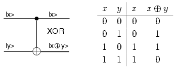
| Figure 1.
A quantum mechanical version of the classical XOR
gate as an
example of a quantum gate (a CNOT gate).
The input state |
Among the main practical problems one has to overcome in the implementation of quantum algorithms are non-ideal performances of the quantum gates [10] involved and random environmental influences, both of which tend to affect the relevant quantum coherence. To protect quantum computation against such errors, two major strategies have been proposed recently, namely active quantum error correction [11]-[19] and passive error avoiding quantum codes [20]-[24]. Active quantum error correction may be viewed as a generalization of classical error correction techniques to the quantum domain. Typically, active quantum error correction involves a properly chosen sequence of frequently repeated measurements. The approach of the error avoiding quantum codes is different. The main idea is to encode the logical information in one of those subspaces of the relevant Hilbert space which is not affected by the physical interactions responsible for the occurrence of errors [20]-[24]. Both theoretical approaches to error correction rely on the concept of redundancy, which is also fundamental for classical error correcting codes [25]. It is expected that error avoiding codes will offer more effective means for stabilizing quantum algorithms. This expectation is based on two facts. Firstly, there is no need for control measurements which are an essential ingredient of any active error correcting code. Secondly, in many cases a smaller number of physical qubits is needed for the representation of a given number of logical qubits.
In the subsequent discussion it is demonstrated that this is indeed the case. By considering Grover's quantum search algorithm it is shown that non-ideal perturbations may be corrected dynamically in an efficient way with the help of an appropriate error avoiding quantum code. By generalizing recent perturbative results [26], it is demonstrated that error avoiding quantum codes may be applicable well beyond the type of errors for which they were originally designed. As a particular example, we discuss coherent errors which may arise from systematic detunings of the physical qubits of the quantum computer from the frequency of the light pulses which realize the required quantum gates. The corresponding error avoiding quantum code with the lowest degree of redundancy is more efficient at encoding quantum information than is any possible active error correcting code which saturates the quantum Hamming bound. The error avoiding quantum code [20] used consists solely of states which are factorizable in the computational basis. In this respect it differs significantly from the recently proposed error avoiding code of [21], for example, which also involves entangled states. Such factorizable codes may offer practical advantages insofar as the implementation of quantum gates in error avoiding subspaces is concerned.
The paper is organized as follows. In section 2 basic facts about Grover's quantum search algorithm are summarized. It is demonstrated that, for large databases, the dynamics of this quantum algorithm can be described by a two-level Hamiltonian which implies that there are Rabi oscillations between the initial state and the sought state. In section 3 general ideas underlying the construction of error avoiding quantum codes are discussed. An efficient error avoiding quantum code which is capable of stabilizing Grover's algorithm against a particular class of coherent errors is presented. The redundancy of this code is discussed and compared with that resulting from active error correcting codes which saturate the quantum Hamming bound. Numerical examples demonstrating the stabilizing capabilities of this error avoiding quantum code are presented in section 4.
2. Grover's quantum search algorithm
Consider an unsorted database with N items and a certain item x0 for which you are searching. As a particular example you can imagine a telephone directory with N entries and a particular telephone number x0 for which you are looking. Furthermore, assume that you are given a black box, i.e. a so-called oracle, which can decide whether an item is x0. Thus, in mathematical terms you are given a Boolean function
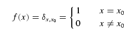 |
(1) |
with
![]() denoting the Kronecker delta function.
Usually the
elements x of the database are assumed to be described by the
N integers
between zero and N-1. Assuming that each application of the oracle
requires
one elementary step, a classical random search process will require
N-1
steps in the worst case and one step in the best possible case. Thus, on
average a classical algorithm will need N/2 steps to find the sought
item x0. It has been shown by Grover [3,4] that, with the
help of his quantum search algorithm, this task can be performed in
denoting the Kronecker delta function.
Usually the
elements x of the database are assumed to be described by the
N integers
between zero and N-1. Assuming that each application of the oracle
requires
one elementary step, a classical random search process will require
N-1
steps in the worst case and one step in the best possible case. Thus, on
average a classical algorithm will need N/2 steps to find the sought
item x0. It has been shown by Grover [3,4] that, with the
help of his quantum search algorithm, this task can be performed in ![]() steps with a probability arbitrarily close to unity. The
basic idea of
this quantum algorithm is to rotate the initial state of the quantum
computation in the direction of the sought state
steps with a probability arbitrarily close to unity. The
basic idea of
this quantum algorithm is to rotate the initial state of the quantum
computation in the direction of the sought state ![]() by a sequence
of unitary quantum versions of the oracle. It will become apparent from the
subsequent discussion that, apart from Hadamard transformations, the dynamics
of this rotation is analogous to a Rabi oscillation between the initially
prepared state and the sought state
by a sequence
of unitary quantum versions of the oracle. It will become apparent from the
subsequent discussion that, apart from Hadamard transformations, the dynamics
of this rotation is analogous to a Rabi oscillation between the initially
prepared state and the sought state ![]() . It has
been shown by Zalka
[27] that Grover's quantum search algorithm is
optimal.
. It has
been shown by Zalka
[27] that Grover's quantum search algorithm is
optimal.
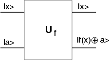
| Figure 2.
A schematic representation of the quantum
oracle |
2.1. The characteristic gate sequence of Grover's search algorithm
In Grover's quantum search algorithm every element of the database is
represented by a state of the computational basis of the quantum computer.
Thus a database which is represented by m qubits has
N = 2m distinguishable
elements. The state
![]() of the computational
basis, for
example, corresponds to the element
0...0110...0 of the database in binary
notation. The quantum oracle
of the computational
basis, for
example, corresponds to the element
0...0110...0 of the database in binary
notation. The quantum oracle ![]() (see figure 2) is determined completely by the
Boolean function of equation (1) and is
represented by a quantum
gate, i.e. by the unitary and Hermitian transformation
(see figure 2) is determined completely by the
Boolean function of equation (1) and is
represented by a quantum
gate, i.e. by the unitary and Hermitian transformation
| |
(2) |
Thereby ![]() is an arbitrary element of the computational
basis and
is an arbitrary element of the computational
basis and
![]() is the state of an additional ancillary qubit
which is discarded
later. The symbol
is the state of an additional ancillary qubit
which is discarded
later. The symbol ![]() denotes addition modulo 2. This unitary
form of the
oracle depends on the Boolean function f(x). Insofar as
complexity estimates
are concerned, it is assumed that this unitary transformation requires one
elementary step. This assumption is analogous to the complexity estimate of
the corresponding classical version of this search problem.
denotes addition modulo 2. This unitary
form of the
oracle depends on the Boolean function f(x). Insofar as
complexity estimates
are concerned, it is assumed that this unitary transformation requires one
elementary step. This assumption is analogous to the complexity estimate of
the corresponding classical version of this search problem.
For the subsequent discussion it is important to note that the elementary
rotations in the direction of the sought quantum state ![]() which are
the key ingredient in Grover's algorithm can be performed with the help of
this unitary oracle. Thus such a rotation can be performed without explicit
knowledge of the state
which are
the key ingredient in Grover's algorithm can be performed with the help of
this unitary oracle. Thus such a rotation can be performed without explicit
knowledge of the state ![]() . Implicit knowledge of it
through the
values of the Boolean function f(x) is sufficient. For
large values of N
it turns out that the number of elementary rotations needed to prepare the
state
. Implicit knowledge of it
through the
values of the Boolean function f(x) is sufficient. For
large values of N
it turns out that the number of elementary rotations needed to prepare the
state ![]() is
is ![]() . To implement such an elementary rotation
from the initial state
. To implement such an elementary rotation
from the initial state
![]() , for example, towards
the final state
, for example, towards
the final state ![]() two different types of quantum gates
are needed,
namely Hadamard gates and controlled phase inversions.
two different types of quantum gates
are needed,
namely Hadamard gates and controlled phase inversions.
A Hadamard gate is a unitary one-qubit operation. It produces an
equally
weighted superposition of the two basis states according to the rule
 |
(3) |
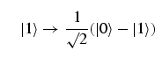 |
(4) |
or, in matrix notation,
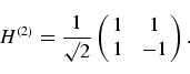 |
An m-qubit Hadamard
gate H(2m) is defined by the
m-fold tensor
product, i.e.
![]() . Thus,
for two
qubits, for example, H(22) is represented
by the matrix
. Thus,
for two
qubits, for example, H(22) is represented
by the matrix
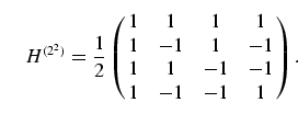 |
(5) |
The Hadamard transformation is Hermitian and unitary. An arbitrary matrix
element
H(2m)i,j of a
Hadamard transformation may be written in the
general form
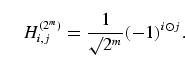 |
(6) |
Here i and j denote binary numbers and the
multiplication ![]() is
bitwise modulo 2, i.e. for i = 1, j = 3 and m
= 2, one obtains
is
bitwise modulo 2, i.e. for i = 1, j = 3 and m
= 2, one obtains
![]() . It has been shown by Grover [3,4] that this
Hadamard transformation can be replaced by any other unitary one-qubit
operation.
. It has been shown by Grover [3,4] that this
Hadamard transformation can be replaced by any other unitary one-qubit
operation.
The remaining quantum gates needed for the implementation of the necessary
rotation are controlled phase inversions with respect to the initial
and
sought states
![]() and
and ![]() . A
controlled
phase inversion with respect to a state
. A
controlled
phase inversion with respect to a state ![]() changes the
phase of this
particular state by an amount
changes the
phase of this
particular state by an amount ![]() and leaves all other states unchanged.
Thus the phase inversion Is with respect to the
initial state
and leaves all other states unchanged.
Thus the phase inversion Is with respect to the
initial state ![]() is defined by
is defined by
 |
(7) |
For two qubits, for example, its matrix representation is given by
 |
(8) |
The controlled phase inversion Ix0 with
respect to the sought
state ![]() is defined in an analogous way. Because the
state
is defined in an analogous way. Because the
state ![]() is not known explicitly but only implicitly
through the
property f(x0) = 1, this transformation
has to be performed with the help of
the quantum oracle. This task can be achieved by preparing the ancillary of
the oracle of equation (2) in the
state
is not known explicitly but only implicitly
through the
property f(x0) = 1, this transformation
has to be performed with the help of
the quantum oracle. This task can be achieved by preparing the ancillary of
the oracle of equation (2) in the
state
![]() . As a consequence one
obtains the required properties
for the phase inversion Ix0, namely
. As a consequence one
obtains the required properties
for the phase inversion Ix0, namely
 |
(9) |
One should bear in mind that this controlled phase inversion can be performed
with the help of the quantum oracle of equation (2) only without
explicit knowledge of the state ![]() .
.
Grover's algorithm starts by preparing all m qubits of the
quantum computer
in the state
![]() . An elementary rotation in the
direction of the sought state
. An elementary rotation in the
direction of the sought state ![]() with the property
f(x0) = 1 is
achieved by the gate sequence
with the property
f(x0) = 1 is
achieved by the gate sequence
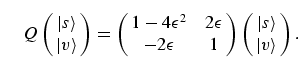
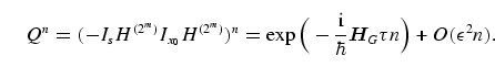
| Q = - Is H(2m) Ix0 H(2m). | (10) |
In order to rotate the initial state![]() into the
state
into the
state ![]() one has to perform a sequence of n such
rotations and a final Hadamard
transformation at the end, i.e.
one has to perform a sequence of n such
rotations and a final Hadamard
transformation at the end, i.e.
| |
(11) |
The effect of the elementary rotation Q is demonstrated in
figure 3 for the case of three
qubits, i.e. m = 3. The first
Hadamard transformation H(23) prepares an
equally weighted state. The
subsequent quantum gate Ix0 inverts the
amplitude of the sought
state
![]() . Together with the subsequent Hadamard
transformation and the phase inversion Is, this gate
sequence Q amplifies
the probability amplitude of the sought state
. Together with the subsequent Hadamard
transformation and the phase inversion Is, this gate
sequence Q amplifies
the probability amplitude of the sought state ![]() . In this
particular case an additional Hadamard transformation finally prepares the
quantum computer in the sought state
. In this
particular case an additional Hadamard transformation finally prepares the
quantum computer in the sought state ![]() with a
probability of 0.88.
with a
probability of 0.88.
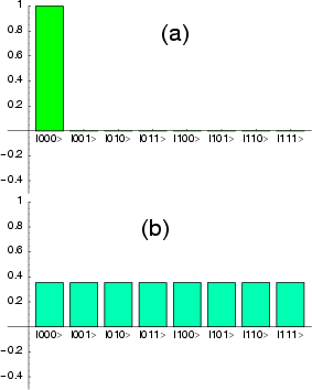
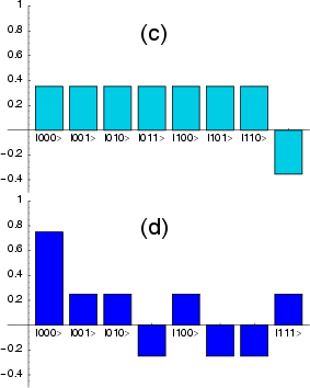
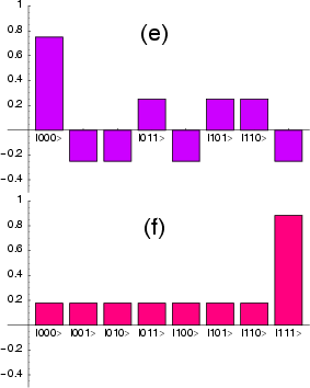
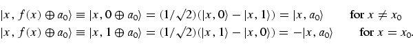
| Figure 3.
Amplitude distributions resulting from the
various quantum gates
involved in Grover's quantum search algorithm for the case of three qubits.
The quantum states which are prepared by these gates are (a)
|
In order to determine the dependence of the ideal number of
repetitions n on
the number of qubits m, it is convenient to analyse the repeated
application
of the gate sequence Q according to equation (11) in terms of the two
states ![]() and
and
![]() whose overlap is
given by
whose overlap is
given by
![]() for m qubits. It is
straightforward to show that the
unitary gate sequence Q preserves the subspace spanned by these
two
states [3,4], i.e.
for m qubits. It is
straightforward to show that the
unitary gate sequence Q preserves the subspace spanned by these
two
states [3,4], i.e.
 |
(12) |
Thus Q acts like a rotation in the plane spanned by
states ![]() and
and ![]() (see figure 4). The angle of rotation is
given by
(see figure 4). The angle of rotation is
given by
![]() .
.
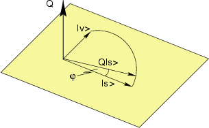
| Figure 4.
Q is a rotation in the subspace spanned by states
|
After j iterations the amplitude of state ![]() is given by
[8]
is given by
[8]
| (13) |
Therefore, the optimal number n of repetitions of the gate sequence Q is approximately given by
 |
(14) |
Finally, it should be mentioned that several generalizations of Grover's original search algorithm which consider arbitrary initial states have also been presented [28,29].
2.2. Hamiltonian representation of Grover's algorithm
If the database contains many elements, i.e.
![]() ,the repeated application of the
elementary rotation which is essential for
Grover's search algorithm can be described by Hamiltonian quantum dynamics
(an
alternative Hamiltonian description has been introduced by Fahri and Gutmann
[30]). The elementary rotation Q can be
approximated by the relation
,the repeated application of the
elementary rotation which is essential for
Grover's search algorithm can be described by Hamiltonian quantum dynamics
(an
alternative Hamiltonian description has been introduced by Fahri and Gutmann
[30]). The elementary rotation Q can be
approximated by the relation
| (15) |
which involves the Hamiltonian
 |
(16) |
The elementary time ![]() might be interpreted as the physical time
required
for performing the elementary rotation Q. The Hamiltonian of
equation (16) describes the
dynamics of a quantum mechanical
two-level system whose degenerate energy levels
might be interpreted as the physical time
required
for performing the elementary rotation Q. The Hamiltonian of
equation (16) describes the
dynamics of a quantum mechanical
two-level system whose degenerate energy levels ![]() and
and ![]() are coupled by a time-independent perturbation. To
lowest order of
are coupled by a time-independent perturbation. To
lowest order of ![]() these degenerate energy levels are
orthogonal. The resulting oscillations
between these coupled energy levels are characterized by the Rabi frequency
these degenerate energy levels are
orthogonal. The resulting oscillations
between these coupled energy levels are characterized by the Rabi frequency
![]() . Correspondingly, the
repeated
application of the elementary rotation Q can be determined with
the help of
Trotter's product formula [31], namely
. Correspondingly, the
repeated
application of the elementary rotation Q can be determined with
the help of
Trotter's product formula [31], namely
 |
(17) |
Thus, in the framework of this Hamiltonian description, applying the
elementary rotation Q n times is equivalent to a
temporal evolution of the
effective two-level quantum system over a time interval of
magnitude ![]() . This Hamiltonian description demonstrates that
the physics behind Grover's
quantum search algorithm is the same as the physics governing the Rabi
oscillations between degenerate or resonantly coupled energy eigenstates.
Since the errors entering equation (17)
are of order
. This Hamiltonian description demonstrates that
the physics behind Grover's
quantum search algorithm is the same as the physics governing the Rabi
oscillations between degenerate or resonantly coupled energy eigenstates.
Since the errors entering equation (17)
are of order
![]() , this Hamiltonian description is applicable only as long
as
, this Hamiltonian description is applicable only as long
as
![]() . Thus, for a given size of the
database, it is valid only
as long as the number of iterations is sufficiently small, i.e.
. Thus, for a given size of the
database, it is valid only
as long as the number of iterations is sufficiently small, i.e. ![]() . However, because Grover's search algorithm needs
approximately
. However, because Grover's search algorithm needs
approximately
![]() steps to find the sought item, the main condition
which
restricts the validity of this Hamiltonian description is a large size of the
database, i.e.
steps to find the sought item, the main condition
which
restricts the validity of this Hamiltonian description is a large size of the
database, i.e.
![]() .
.
| Figure 5.
The probability of being in the state |
2.3. An example of coherent errors
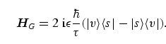
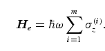
So far we have been concentrating on the ideal dynamics of Grover's quantum search algorithm. However, in practical applications it is very difficult to realize this search algorithm in an ideal way. Usually the ideal dynamics is affected by numerous perturbations. Physically one may distinguish two different kinds of errors, namely incoherent and coherent ones. Typically incoherent perturbations originate from a coupling of the physical qubits of a quantum computer to an uncontrollable environment. As a consequence the resulting errors are of a stochastic nature. Coherent errors may arise from non-ideal quantum gates which lead to a unitary but non-ideal temporal evolution of the quantum algorithm. A simple example of this type of errors is systematic detuning from resonance of the light pulses with which the required quantum gates are realized on the physical qubits. In the Hamiltonian formulation of Grover's algorithm such systematic detunings may be described by a perturbing Hamiltonian of the form
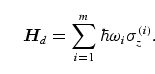 |
(18) |
In equation (18) it has been assumed that
Grover's quantum algorithm
is realized by m qubits and that the ith qubit is detuned
with respect to
the ideal transition frequency by an amount ![]() . A possible
result is shown in
figure 5. The Pauli
spin-operator of the ith qubit is denoted
. A possible
result is shown in
figure 5. The Pauli
spin-operator of the ith qubit is denoted
![]() . In the presence
of these systematic detunings and for a large number of qubits the dynamics
of
Grover's algorithm is described by the Hamiltonians of
equations (16) and (18).
. In the presence
of these systematic detunings and for a large number of qubits the dynamics
of
Grover's algorithm is described by the Hamiltonians of
equations (16) and (18).
In order to obtain insight into the influence of this type of coherent
errors,
the performance of Grover's algorithm under repeated applications of the
elementary rotation Q is depicted in figure 5. The dynamics of
the ideal Grover algorithm for the case of three qubits, i.e. m =
3, is
depicted by the broken line. The Rabi oscillations with frequency
![]() are clearly visible. The
full line shows the
probability of observing the quantum computer in the state
are clearly visible. The
full line shows the
probability of observing the quantum computer in the state ![]() in a
case in which all the qubits are detuned from their ideal resonance
frequency.
One notices the deviations from the ideal behaviour. Owing to the coherent
nature of the errors, the temporal evolution of the non-ideal algorithm
exhibits revival phenomena [32].
in a
case in which all the qubits are detuned from their ideal resonance
frequency.
One notices the deviations from the ideal behaviour. Owing to the coherent
nature of the errors, the temporal evolution of the non-ideal algorithm
exhibits revival phenomena [32].
3. Error avoiding quantum codes
In general there are two different strategies for correcting errors in quantum information processing. Active quantum error correcting schemes may be viewed as generalizations of classical error correction techniques to the quantum domain [11]-[14]. Typically they involve a suitably chosen quantum code and a sequence of quantum measurements. A non-degenerate code, which is the simplest example, has to map all possible states which may result from arbitrary environmental influences onto orthogonal states. According to basic postulates of quantum theory these orthogonal quantum states can be distinguished and, from the result of a control measurement, one may restore the original quantum state. So far these general techniques have been applied mainly to the stabilization of static quantum memories [33].
The second possible error correction strategy, which seems to be suitable
also
for stabilizing quantum algorithms, is based on error avoiding quantum
codes [20]-[24]. These latter methods rely on knowledge of
basic properties of
the relevant error. The main idea is to encode the quantum information in
those subspaces of the Hilbert space which are not affected by the errors.
This aim is achieved by restricting oneself to degenerate eigenspaces of the
relevant error operators. Thus, in the special case of a single error
operator, say E, the basis states
![]() of such an
error-free subspace have to satisfy the relation
of such an
error-free subspace have to satisfy the relation
| |
(19) |
Error avoiding quantum codes are completely degenerate error correcting codes
in the sense that the code space is preserved under the influence of the
errors and therefore no recovery operation is needed [34]. In the
above-mentioned example of coherent errors which may affect Grover's
algorithm
this error operator is given by the Hamiltonian of equation (18),
i.e.
E =
Hd. It is crucial for the success of
an error avoiding
code that the eigenvalue c of equation (19) does not depend on the
states belonging to the error-free subspace. This implies that all possible
elements of the error-free subspace of the general form
![]() are affected by the error operator in
the same way, i.e.
are affected by the error operator in
the same way, i.e.
 |
(20) |
It is apparent that a non-trivial error avoiding code is possible only if the eigenspace of the error operator E is degenerate.
3.1. An error avoiding quantum code stabilizing coherent errors
As an example of an error avoiding quantum code let us consider the case of
coherent errors which may affect Grover's quantum algorithm and which can be
characterized by the
Hamiltonian Hd of
equation (18). In the
simple case of equal detunings, i.e.
![]() ,the error
operator E reduces to the form
,the error
operator E reduces to the form
 |
(21) |
It is easy to find highly degenerate error-free subspaces of this error
operator. All states with a fixed number of ones and zeros constitute a
degenerate eigenspace of He [34,35]. For an even number
of qubits it is possible to find an error avoiding subspace with eigenvalue
c = 0 so that
| (22) |
for all elements
![]() of this subspace. For this purpose
one is
looking for quantum states with zero total spin. For four qubits, for
example,
this subspace is defined by the basis vectors
of this subspace. For this purpose
one is
looking for quantum states with zero total spin. For four qubits, for
example,
this subspace is defined by the basis vectors
![]() ,
,
![]() ,
,
![]() ,
,
![]() ,
,
![]() and
and
![]() and involves all states with the same number of
zeros and ones. Four
of these states may be used as a basis for the state space of two
logical qubits. For these eigenstates the error Hamiltonian
He maps
onto zero, e.g.
and involves all states with the same number of
zeros and ones. Four
of these states may be used as a basis for the state space of two
logical qubits. For these eigenstates the error Hamiltonian
He maps
onto zero, e.g.
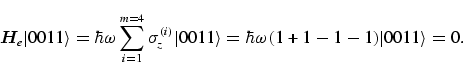 |
This particular error avoiding code works ideally for equal detunings of all qubits from resonance. It is formed by quantum states which factorize in the computational basis. So it is expected that the encoding of quantum information and the implementation of quantum gates in this error-free subspace will be considerably easier than will that in cases in which the error avoiding codes involve entangled quantum states.
3.2. Implementation of quantum gates in an error-free subspace
To realize a quantum algorithm in an error-free subspace one has to implement
the necessary quantum gates in such a way that they do not mix the error-free
subspace with its orthogonal complement [36,37]. Consider two
logical qubits, for example, which are encoded by four physical qubits. For
this purpose one may choose the states
![]() ,
,
![]() ,
,
![]() and
and
![]() which have been mentioned in the previous
subsection. This error avoiding code works ideally for stabilizing Grover's
algorithm with respect to the error operator
He of
equation (21) provided that it is possible
to realize the required
unitary transformations, namely Hadamard transformations and the controlled
phase inversions.
which have been mentioned in the previous
subsection. This error avoiding code works ideally for stabilizing Grover's
algorithm with respect to the error operator
He of
equation (21) provided that it is possible
to realize the required
unitary transformations, namely Hadamard transformations and the controlled
phase inversions.
Consider as an example a Hadamard transformation which acts in a
two-dimensional error avoiding subspace of this kind. Hence it is assumed
that
the two basis states of this error avoiding code are given by ![]() and
and
![]() and that they involve two physical qubits. Thus,
we are looking
for a transformation which performs the mappings
and that they involve two physical qubits. Thus,
we are looking
for a transformation which performs the mappings
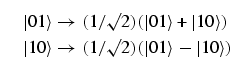 |
(23) |
and which does not mix the subspace spanned by ![]() and
and ![]() with the orthogonal space spanned by the basis
states
with the orthogonal space spanned by the basis
states ![]() and
and
![]() . In matrix notation we are looking for a unitary
matrix of the
form
. In matrix notation we are looking for a unitary
matrix of the
form
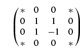 |
(24) |
with ![]() denoting arbitrary entries which ensure
unitarity. Such a
transformation can be achieved by the gate sequence
denoting arbitrary entries which ensure
unitarity. Such a
transformation can be achieved by the gate sequence
![]() with
with
![]() . Here
CNOT21 is a controlled-not operation with the first
qubit as the
target and the second qubit as the control qubit and
. Here
CNOT21 is a controlled-not operation with the first
qubit as the
target and the second qubit as the control qubit and ![]() is the Pauli
matrix. Thus in matrix notation this relation yields
is the Pauli
matrix. Thus in matrix notation this relation yields
 |
(25) |
Obviously the final result does not mix the error avoiding subspace with its orthogonal complement. However, such a mixing might take place in the intermediate steps, depending on which set of universal quantum gates can be implemented. However, even in the worst possible case it suffices to ensure that the time spent by the quantum computer in the orthogonal complement of the error avoiding subspace is sufficiently small that the resulting errors can be neglected for all practical purposes. Under these circumstances it is expected that the implementation of quantum algorithms in error avoiding subspaces will be a powerful means for stabilizing quantum codes.
3.3. Code sizes of error avoiding quantum codes
In order to estimate the redundancy which has to be introduced for
stabilizing
a quantum algorithm by an error avoiding quantum code let us consider the
particular example of section 3.1 in more detail. It has been argued
that, in
the case of coherent errors which can be characterized by the Hamiltonian of
equation (21), an error avoiding quantum
code can be constructed from
basis states with equal numbers of ones and zeros. In order to minimize the
redundancy it is desirable to maximize the dimension of the resulting error
avoiding subspace. If one starts with m physical qubits, the
dimension D(m,q) of the corresponding error
avoiding subspace with
q qubits in state ![]() and
m - q qubits in state
and
m - q qubits in state ![]() , for
example, is given by
, for
example, is given by
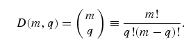 |
(26) |
From elementary properties of binomial coefficients it is clear that
D(m,q) is maximum for
q = m/2. Thus, for an even number of
qubits m, the
largest possible dimension of the resulting error avoiding subspace is given
by
![\begin{equation}
D(m,m/2) = \frac{m!}{[(m/2)!]^2} \to
2^m\left(\frac{2}{m\pi}\right)^{\!1/2}\tqs (m\gg
1).
\end{equation}](grover/img107.gif) |
(27) |
Thus, in this case it is possible to encode
![\begin{equation}
l = {\rm log}_2 D(m,m/2) \to m - \frac{{\rm log}_2 m}{2}
+{\rm log}_2[(2/\pi)^{1/2}]\tqs (m\gg
1)
\end{equation}](grover/img108.gif) |
(28) |
logical qubits with m physical ones. It is instructive to compare the redundancy of this error avoiding code described by equation (28) with the ones resulting from active error correcting quantum codes which saturate the quantum Hamming bound [13,25]. If one wants to correct arbitrary errors of maximum length t with a non-degenerate error correcting quantum code, the number of physical and logical qubits m and l must satisfy the so-called quantum Hamming bound [13,14,25], i.e.
 |
(29) |
Here the length t of an error is the number of one-qubit errors which
can be
detected by a single measurement and which can thus be corrected; ![]() is the
number of different one-qubit errors the code is able to correct. This
inequality reflects the fact that, in a non-degenerate error correcting
quantum code, the actions of various error operators on any of the logical
qubits must lead to orthogonal quantum states. The dimension of the resulting
Hilbert space described by the left-hand side of the
inequality (29) has to be smaller than
the dimensions of the
Hilbert spaces of all physical qubits. For the detuning given by (21),
there is only one error, i.e.
is the
number of different one-qubit errors the code is able to correct. This
inequality reflects the fact that, in a non-degenerate error correcting
quantum code, the actions of various error operators on any of the logical
qubits must lead to orthogonal quantum states. The dimension of the resulting
Hilbert space described by the left-hand side of the
inequality (29) has to be smaller than
the dimensions of the
Hilbert spaces of all physical qubits. For the detuning given by (21),
there is only one error, i.e. ![]() . Thus the number of logical
qubits
obtainable by a non-degenerate error correcting code of maximum length unity,
i.e. t = 1, cannot be larger than
. Thus the number of logical
qubits
obtainable by a non-degenerate error correcting code of maximum length unity,
i.e. t = 1, cannot be larger than
| l;SPMgt; = m - log2(m+1). | (30) |
On comparing equation (28) with
equation (30), one realizes
that the redundancy of this particular error avoiding quantum code is smaller
than that of any non-degenerate error correcting code saturating the
Hamming bound, i.e.
 |
(31) |
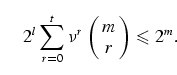
For codes with maximum lengths larger than 1, we obtain
![]() log2 m (see figure 6). An error avoiding code may be considered
as an error correcting
code which is capable of correcting errors of infinite length, i.e.
log2 m (see figure 6). An error avoiding code may be considered
as an error correcting
code which is capable of correcting errors of infinite length, i.e. ![]() [38]. In addition, its redundancy is smaller
than that of a
non-degenerate code which is able to correct only errors of distance t
= 1.
[38]. In addition, its redundancy is smaller
than that of a
non-degenerate code which is able to correct only errors of distance t
= 1.
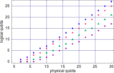
| Figure 6. The maximum number of logical qubits l versus the number of physical qubits m for the error avoiding quantum codes which are capable of stabilizing the error operator of equation (21) (diamonds) (compare with equation (28)). The corresponding relation l > (m) obtained from equation (29) characterizing the quantum Hamming bound is indicated by stars (t = 1), triangles (t = 2) and boxes (t = 3). |
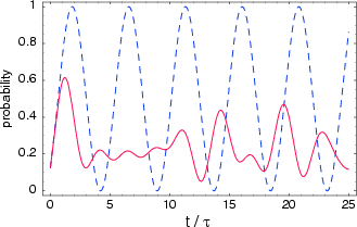
In the previous section we have developed an error avoiding quantum code which is capable of correcting coherent errors. These errors were assumed to be caused by systematic detunings of the physical qubits of the quantum computer from the frequency of the laser pulses implementing the action of the quantum gates. This error avoiding quantum code works perfectly provided that all physical qubits are detuned from the frequency of these laser pulses by the same amount. However, in realistic situations this case is hardly ever realized. For the realistic assumption of unequal detunings in general the eigenstates of Hd are non-degenerate so that it is not possible to construct a perfect error avoiding quantum code. Therefore the practical question of whether the presented error avoiding quantum code of section 3 is still useful for stabilizing quantum algorithms against arbitrary systematic detunings arises. A first general result in this direction was derived by Lidar et al [26]. They have shown in a perturbative analysis that any error avoiding quantum code is stable against weak perturbations. However, so far questions concerning the maximal range of validity of an error avoiding quantum code have not been addressed.
| Figure 7.
The probability of finding the quantum computer
in the sought
state |
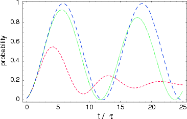
The dynamics of Grover's algorithm in the presence of arbitrary detunings is
depicted in figure 7. The broken line
represents the ideal
dynamics in the absence of detunings for the case of six qubits
evaluated from
the Hamiltonian of equation (16).
The characteristic Rabi
oscillations are clearly apparent. The corresponding dynamics for
eight qubits
in the presence of arbitrarily chosen detunings is depicted by the dotted
line
in figure 7. It is apparent that, in
this case, a quantum search
for the state ![]() is not at all successful. However,
as is apparent
from the full line in figure 7,
encoding the quantum information
by the error avoiding code of section 3
improves the performance considerably.
Despite the fact that this error avoiding code has not been designed for
these
detunings, it almost succeeds at finding the sought quantum
state
is not at all successful. However,
as is apparent
from the full line in figure 7,
encoding the quantum information
by the error avoiding code of section 3
improves the performance considerably.
Despite the fact that this error avoiding code has not been designed for
these
detunings, it almost succeeds at finding the sought quantum
state ![]() after a number of iterations which is close to
that of the
ideal case (compare with equation (14)). Similar stability
properties of error avoiding codes have been observed by Lidar et al
[26].
after a number of iterations which is close to
that of the
ideal case (compare with equation (14)). Similar stability
properties of error avoiding codes have been observed by Lidar et al
[26].
In order to obtain more insight into the stabilizing properties of this error
avoiding code, let us investigate the probability of success in the presence
of arbitrary detunings in more detail. For this purpose we consider eight
physical qubits whose detunings ![]() are distributed
randomly according
to a normal distribution. According to figure 6 these eight
physical qubits are capable of encoding six logical qubits. In
figure 8 the average value of the
maximum probability of finding
the quantum computer in the sought state
are distributed
randomly according
to a normal distribution. According to figure 6 these eight
physical qubits are capable of encoding six logical qubits. In
figure 8 the average value of the
maximum probability of finding
the quantum computer in the sought state ![]() for
various values of
the variance of the randomly chosen detunings is depicted. The lower sequence
of dots (stars) refers to Grover's algorithms without error avoiding encoding
and the upper sequence of points (diamonds) refers to error avoiding encoding
according to section 3. It is apparent that
error avoiding encoding is very
successful as long as the difference between the detunings of the qubits is
sufficiently small. Only in extreme cases in which these differences become
comparable to the typical magnitudes of the detunings is this type of error
avoiding code no longer capable of stabilizing Grover's algorithm in a
satisfactory way.
for
various values of
the variance of the randomly chosen detunings is depicted. The lower sequence
of dots (stars) refers to Grover's algorithms without error avoiding encoding
and the upper sequence of points (diamonds) refers to error avoiding encoding
according to section 3. It is apparent that
error avoiding encoding is very
successful as long as the difference between the detunings of the qubits is
sufficiently small. Only in extreme cases in which these differences become
comparable to the typical magnitudes of the detunings is this type of error
avoiding code no longer capable of stabilizing Grover's algorithm in a
satisfactory way.
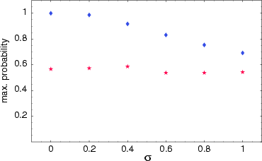
| Figure 8.
The average maximum probability of success for
Grover's algorithm
with eight qubits in the presence of randomly chosen detunings: with
error
avoiding encoding according to section 3
(diamonds); and without error
avoiding encoding (stars). The detunings |
It has been demonstrated that error avoiding quantum codes may offer efficient methods for stabilizing quantum codes dynamically against errors. As a particular example we discussed the stabilization of Grover's quantum search algorithm against coherent errors which may arise from systematic detunings of the physical qubits from the frequency of the light pulses implementing the quantum gates. Even though originally the error avoiding quantum code had been constructed for the special case of equal detunings of all the qubits, it has been shown that it is also capable of stabilizing this quantum algorithm to a satisfactory degree in other non-ideal cases well beyond the perturbative regime. The error avoiding quantum code considered consists solely of quantum states which are factorizable in the computational basis. This may offer advantages insofar as the implementation of the necessary quantum gates in this error-free subspace is concerned. Although the stabilizing ability of error avoiding quantum codes has been demonstrated for one particular quantum code and one particular class of coherent errors only, it is expected that similar capabilities will also be found in more general cases which may also involve incoherent errors.
After the submission of this paper we became aware of a preprint by Kempe et al [39] concerning quantum computation on decoherence-free subspaces. In this preprint some of the issues addressed in section 3.2 are also considered.
This work was supported by the DFG within the SPP `Quanteninformationsverarbeitung'. Stimulating discussions with Thomas Beth, Markus Grassl and Dominik Janzing are acknowledged. AD acknowledges support by the DAAD.
| This volume |
|
| Copyright © 1998-2005 Deutsche Physikalische Gesellschaft & Institute of Physics |