


Next: Asymptotic properties of the
Up: The Skyrme Hartree-Fock-Bogolyubov equations
Previous: The Hartree-Fock-Bogolyubov mean fields
The Hartree-Fock-Bogolyubov equations
Writing the fields in matrix form
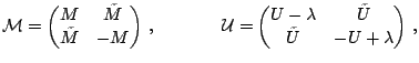 |
(30) |
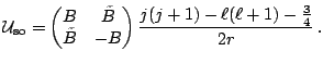 |
(31) |
The HFB equations read
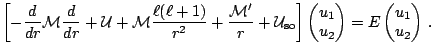 |
(32) |
An  -dependant mixing of components and scaling described
in Ref. [5] allows us to write this
equation as an equation with no differential operator in
the coupling terms and no first order derivative
-dependant mixing of components and scaling described
in Ref. [5] allows us to write this
equation as an equation with no differential operator in
the coupling terms and no first order derivative
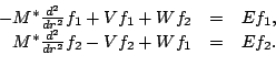 |
(33) |
This last form with no first order derivative of the functions
is particularly suitable for the numerical integration by the
Numerov algorithm briefly discussed in section 5.2.
Jacek Dobaczewski
2005-01-23