Method

Our first step in the self-consistent treatment of excitations is to solve the spherical HFB equations in coordinate space (without mixing neutron and proton quasiparticle wave functions [63]), with the method developed in Ref. [64] (see also Refs. [60,65,66]). We can use arbitrary Skyrme functionals in the particle-hole and pairing (particle-particle) channels.

We modify the code used in Refs. [64,60,65] so that it solves the HFB equations with higher accuracy, which we need because the QRPA uses all the single-quasiparticle states produced by the HFB equations, even those that are essentially unoccupied. Our modifications are: (i) the use of quadruple precision (though in solving the QRPA equations we use double precision); (ii) a smaller discretization length (0.05 fm); and (iii) a high quasiparticle-energy cutoff (200 MeV) and a maximum angular momentum $j_{\rm max}$=15/2 ($N\leq 82$) or 21/2 ($N>82$). In a 20 fm box, this cutoff corresponds to 200-300 quasiparticle states for each kind of nucleon. We include all these quasiparticle states in the HFB calculation because a very large energy cutoff is essential for the accuracy of self-consistent QRPA calculations [10]. Hence, the effective pairing window in our HFB calculations is also very large, with the pairing functional fitted to experimental pairing gaps extracted as in Ref. [67] from the measured odd-even mass differences in several Sn, Ni, and Ca isotopes.

Next, we construct the canonical basis, the eigenstates of single-particle density matrix $\rho$. To avoid poor accuracy (see Ref. [60]) in the wave functions of the nearly empty canonical particle states, we do not diagonalize $\rho$ directly in coordinate space. Instead we construct an intermediate basis by orthonormalizing a set of functions $\{ \varphi^{\mu}_1({\mbox{\boldmath$r$\unboldmath }}) +\varphi^{\mu}_2( {\mbox{\boldmath$r$\unboldmath }})\}$, where $\varphi^{\mu}_1({\mbox{\boldmath$r$\unboldmath }})$ and $\varphi^{\mu}_2( {\mbox{\boldmath$r$\unboldmath }})$ are the upper and lower components of the quasiparticle wave function with energy $E_{\mu}$ [64]. We use the density matrix in coordinate space to calculate the matrix in this basis, which we then diagonalize to obtain the canonical states. The reason for using the sum of $\varphi^{\mu}_1({\mbox{\boldmath$r$\unboldmath }})$ and $\varphi^{\mu}_2( {\mbox{\boldmath$r$\unboldmath }})$ is that solutions of the HFB equations expressed in the canonical basis (Eqs. (4.14) of Ref. [60]) are, in the new basis, guaranteed to be numerically consistent with those of the original HFB problem. This is because the configuration space is the same in both cases, independent of the pairing cutoff (see Ref. [68] for a discussion relevant to this point). Without pairing, when either $\varphi^{\mu}_1({\mbox{\boldmath$r$\unboldmath }})$ or $\varphi^{\mu}_2( {\mbox{\boldmath$r$\unboldmath }})$ is equal to zero, our method is equivalent to taking a certain number of HF states, including many unoccupied states.

In the canonical basis, the HFB+QRPA equations have a form almost identical to that of the BCS+QRPA approximation, the only difference being the presence of off-diagonal terms in the single-quasiparticle energies. The QRPA+HFB formalism employs more pairing matrix elements than the QRPA+BCS, however.

As noted already, full self consistency requires the use of the same interaction in the QRPA as in the HFB approximation. More specifically, this means that the matrix elements that enter the QRPA equation are related to second derivatives of a mean-field energy functional. We describe the densities and the form of the functional carefully in the appendices. But we must meet other conditions as well for QRPA calculation to be self-consistent. Essentially all the single-particle or quasiparticle states produced by the HFB calculation must be used in the space of two-quasiparticle QRPA excitations. This requirement is rather stringent, so we truncate the two-quasiparticle space at several levels and check for convergence of the QRPA solution. First we omit canonical-basis wave functions that have occupation probabilities $v_i^2$ less than some small $v_{\rm crit}^2$, (or HF energies greater than some $\varepsilon _{\rm crit}$ if there is no pairing). Then we exclude from the QRPA pairs of canonical states for which the occupation probabilities are both larger than $1-v_{\rm crit}^2$. This second cut is based on the assumption that two-particle transfer modes are not strongly coupled to particle-hole excitations. In addition, if the factors containing $u_i$ and $v_i$ in the QRPA equation -- see Eqs. (21) and (22) -- are very small, in practice smaller than 0.01, then we set the corresponding matrix elements equal to zero. This does not affect the size of the QRPA space, but significantly speeds up the calculations. For good performance we diagonalize QRPA-Hamiltonian matrices of order $20,000 \times 20,000$ in neutron-rich Sn isotopes.

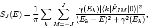
Having solved the QRPA equations, we can then calculate the strength function

$$S_J(E) = \frac{1}{\pi}\sum_{k}\sum_{M=-J}^J\frac{\gamma(E_k)... ...\hat{F}_{JM}\vert 0\rangle\vert^2}{(E_k-E)^2 + \gamma^2(E_k)},$$ (1)

for the multipole operator $\hat{F}_{JM}$. The smoothing width $\gamma$ is supposed to be large enough to remove spurious oscillations in $S_J(E)$ associated with a finite box radius $R_{\rm box}$ [69,55]. A reasonable form, based on a single-particle estimate, for the smoothing width (App. B of Ref. [69]), is

$$\gamma(E)=\left\{\begin{array}{ll} \frac{\pi}{R_{\rm box}}\sqrt{\... ...geq-\lambda_{\rm n} \\ 0.1~{\rm MeV}, & E<-\lambda_{\rm n} \end{array}\right.,$$ (2)

where $\lambda_{\rm n}$ is the neutron Fermi level and $m$ is the nucleon mass. In deriving Eq. (2) we assumed that the single-proton continuum is effectively shifted up several MeV by the Coulomb barrier. In other words, we associate the threshold energy with the neutron Fermi level.

In all the tests below, we use the Skyrme functional SkM$^\ast$ [70] and a volume pairing functional [71] ( $C^{\tilde{\rho}}(\rho_{00})$ a constant in Eq. (34)). The pairing parameter in Eq. (44) is $V_0=-77.5$ MeV fm$^3$. Usually we work in a box of radius 20 fm, though we vary this radius below to see its effects. In several tests we examine the weakly bound nucleus $^{174}$Sn, which is very close to the two-neutron drip line. In this system, the protons are unpaired and the neutrons paired (with $\Delta_{\rm n}$=1.016MeV) in the HFB ground state.