Density matrix expansion with spin and isospin

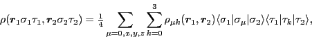
For nucleons, the density matrix $\rho(\bboxr_1\sigma_1\tau_1,\bboxr_2\sigma_2\tau_2)$ depends not only on positions $\bboxr_1$ and $\bboxr_2$ but also on spin $\sigma_1,\sigma_2=\pm1$ and isospin $\tau_1,\tau_2=\pm1$ coordinates. Since the strong two-body interaction is assumed to be isospin and rotationally invariant, it is convenient to represent the standard density matrix $\rho(\bboxr_1\sigma_1\tau_1,\bboxr_2\sigma_2\tau_2)$ through nonlocal densities $\rho_{\mu k}(\bboxr_1,\bboxr_2)$ as:

$$\rho(\bboxr_1\sigma_1\tau_1,\bboxr_2\sigma_2\tau_2) = {\text... ...igma_2\rangle \langle \tau_1\vert \tau_k \vert\tau_2 \rangle ,$$ (39)

where $\sigma_0$ ( $\sigma_{x,y,z}$) and $\tau_0$ ($\tau_{1,2,3}$) are the unity (Pauli) matrices in the spin and isospin coordinates, respectively. For $\mu=0$ and $\mu=x,y,z$, the densities are scalars and vectors, respectively, and for $k=0$ and $k=1,2,3$, they are isoscalars and isovectors, so altogether the density matrix is split into the four standard spin-isospin channels.

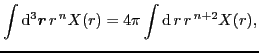
For the direct term, we can proceed as in Sec. 2.1, by making the Taylor expansions of local densities (at $\bboxr_1=\bboxr_2$) in each spin-isospin channel; that is, similarly as in Eqs. (6) and (7), we have

$$\rho_{\mu k}(\mbox{{\boldmath {$R$}}}\pm {\textstyle{\frac{1}{2}}}\mbox{{\boldmath {$r$}}}) = \rho_{\mu k}(\mbox{{\boldmath {$R$}}}) \pm {\textstyle{\frac{1}{2... ...}} r_a r_b \nabla_a\nabla_b\rho_{\mu k}(\mbox{{\boldmath {$R$}}}) + \ldots \,.$$ (40)

For the exchange term, Sec. 2.2, the analogous Taylor expansions of nonlocal densities, similarly as in Eq. (14), read

$$\hspace*{-2cm} \rho_{\mu k}(\mbox{{\boldmath {$R$}}},\pm\mbox{{\boldmath {$r$}}}) = \rho_{\mu k}(\mbox{{\boldmath {$R$}}}) \pm i r_aj_{\mu ak}(\mbox... ...\boldmath {$R$}}})-\tau_{\mu abk}(\mbox{{\boldmath {$R$}}})\right] + \ldots \,,$$ (41)

where the current ( $j_{\mu ak}(\mbox{{\boldmath {$R$}}})$) and kinetic ( $\tau_{\mu abk}(\mbox{{\boldmath {$R$}}})$) densities are defined in each channel as in Eqs. (15), namely,

$$j_{\mu ak}(\mbox{{\boldmath {$R$}}}) ={\textstyle{\frac{1}{... ...a_b^{(2)}\rho_{\mu k}(\bboxr_1,\bboxr_2)_{\bboxr_1=\bboxr_2} .$$ (42)

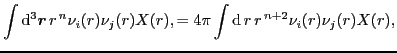
The local density approximation of densities in all channels, analogous to Eqs. (16) and (24), is now postulated as

$$\hspace*{-2cm} \rho_{\mu k}(\mbox{{\boldmath {$R$}}},\pm\mbox{{\boldmath {$r$}}}) = \pi_0(r) \rho_{\mu k}(\mbox{{\boldmath {$R$}}}) \pm i\pi_1(r) r_aj_{\mu ak}(\mbox{{\boldmath {$R$}}})$$

$$+ {\textstyle{\frac{1}{2}}}\pi_2(r) r_a r_b \left[{\textstyle{\f... ...\boldmath {$R$}}})-\tau_{\mu abk}(\mbox{{\boldmath {$R$}}})\right] + \ldots \,,$$ (43)

and

$$\hspace*{-2cm} \rho_{\mu k}(\mbox{{\boldmath {$R$}}},\pm\mbox{{\boldmath {$r$}}}) = \nu_0({r})\rho_{\mu k}(\mbox{{\boldmath {$R$}}}) \pm i\nu_1({r}) r_aj_{\mu ak}\rho(\mbox{{\boldmath {$R$}}})$$

$$+ {\textstyle{\frac{1}{2}}} \nu_2({r}) r_a r_b \left[{\textstyle{... ...1}{5}}}\delta_{ab}k_F^2\rho_{\mu k}(\mbox{{\boldmath {$R$}}})\right] + \ldots~.$$ (44)

At this point, we have assumed that functions $\pi _i(r)$ and $\nu_i(r)$ are channel-independent, that is, that they are scalar-isoscalar functions. In A we discuss this point in more detail, and we show that the postulate of simply channel-dependent functions $\pi _i(r)$ and $\nu_i(r)$ is incompatible with properties of infinite matter, whereas the proper treatment of the problem leads immediately to the channel mixing and the energy density, which is not invariant with respect to rotational and isospin symmetries. This question certainly requires further study, whereas at the moment, a consistent approach can only be obtained by assuming the scalar-isoscalar functions $\pi _i(r)$ and $\nu_i(r)$.

We can now apply derivations presented in Secs. 2.1 and 2.2 to the general case of an arbitrary finite-range local nuclear interaction composed of the standard central, spin-orbit, and tensor terms:

$$\hat V(\bboxr_1,\bboxr_2) = W(r) + B(r) P_\sigma - H(r) P_\tau - M(r) P_\sigma P_\tau$$

$$+ \Big[P(r) + Q(r) P_\tau\Big]\bbox{L}\cdot\bbox{S} + \Big[R(r) + S(r) P_\tau\Big]S_{12},$$ (45)

where $r$= $\vert\mbox{{\boldmath {$r$}}}\vert$=$\vert\bboxr_1$$-$$\bboxr_2\vert$, and

$$P_\sigma={\textstyle{\frac{1}{2}}}(1+\bbox{\sigma}_1\cdot\bb... ...\textstyle{\frac{1}{2}}}(1+\vec {\tau }_1\circ\vec {\tau }_2),$$ (46)

$$\bbox{L}=-i\hbar\mbox{{\boldmath {$r$}}}\times\bbox{\partial... ...mbox{{\boldmath {$r$}}})- \bbox{\sigma}_1\cdot\bbox{\sigma}_2.$$ (47)

After straightforward but lengthy calculations, one obtains the interaction energy in the form of a local integral, analogous to that for the Skyrme interaction [28,22,19],

$${\cal E}^{\text{int}} = \int{\rm d}^3\mbox{{\boldmath {$R$}}}\sum... ...ho} \rho_k\Delta\rho_k + C_t^{\tau} \Big(\rho_k\tau_k - \bbox{j}_k^{\,2}\Big)$$

$$~~~~~~~~~~~~~~~~~~~~~ + C_t^{ s} \bbox{s}_k^{\,2} + C_t^{\Delta... ...{ T} \Big(\bbox{s}_k\cdot\bbox{T}_k - {\mathsf J}_{abk} {\mathsf J}_{abk}\Big)$$

$$~~~~~~~~~~~~~~~~~~~~~ + C_t^{F} \Big(\bbox{s}_k \cdot\bbox{F}_k ... ...athsf J}_{bak}\Big) + C_t^{\nabla{s}} \Big(\bbox{\nabla}\cdot\bbox{s}_k\Big)^2$$

$$~~~~~~~~~~~~~~~~~~~~~ + C_t^{\nabla{J}} \Big(\rho_k\bbox{\nabla}\cdot\bbox{J}_k + \bbox{s}_k\cdot(\bbox{\nabla}\times\bbox{j}_k)\Big) \Bigg],$$ (48)

where $\rho_k \equiv\rho_{0k}$, $\tau_k \equiv\tau_{0bbk}$, $\bbox{j}_{ak} \equiv j_{0ak}$, $\bbox{s}_{ak} \equiv \rho_{ak}$, $\bbox{T}_{ak} \equiv\tau_{abbk}$, $\bbox{F}_{ak} \equiv{\textstyle{\frac{1}{2}}}(\tau_{babk}+\tau_{bbak})$, ${\mathsf J}_{abk} \equiv j_{abk}$, and $\bbox{J}_{ak} \equiv \epsilon_{abc}j_{cbk}$ are the standard local densities. The isoscalar ($t=0$) and isovector ($t=1$) coupling constants $C_t$ correspond to $k=0$ and $k=1,2,3$, respectively.

The coupling constants of the local energy density (48) are related to moments of the interaction in the following way:

$$\hspace*{-2cm} 8\left(\begin{array}{l}C_0^{\rho}\\ C_1^{\rho}\\ C_0^{ s}\\ C_1^{ s}\end{array}\right) = \left(\begin{array}{r@{\hspace{\sep}}r@{\hspace{\sep}}r@{\hspace{... ...{00}_{\nu0}+{\textstyle{\frac{1}{5}}}W^{02}_{\nu2}\,k_F^2 \end{array}\right) ,$$ (49)

$$\hspace*{-2cm} 96\left(\begin{array}{l}C_0^{\Delta\rho}\\ C_1... ... F} \\ C_1^{ F} \\ C_0^{\nabla s} \\ C_1^{\nabla s} \end{array}\right) = \left(\begin{array}{r@{\hspace{\sep}}r@{\hspace{\sep}}r@{\hspace{... ... { {\frac{4}{5}}}S _2 \\ { {\frac{4}{5}}}S^{02}_{\nu2} \end{array}\right) ,$$ (50)

$$\hspace*{-2cm} 24\left(\begin{array}{l}C_0^{\nabla{J}}\\ C_1^{\nabla{J}}\end{array}\right) = \left(\begin{array}{rr} 2 & 1 \\ 0 & 1 \end{array}\right) \left(\begin{array}{c}P_2+Q^{01}_{\nu2}\\ Q_2+P^{01}_{\nu2} \end{array}\right) .$$ (51)

All the coupling constants of the local energy density (48) depend linearly on the following moments of potentials:

$$X_n = \int{\rm d}^3\mbox{{\boldmath {$r$}}}\, r^{\,n} X(r) = 4\pi\int{\rm d}\,r\, r^{\,n+2} X(r) ,$$ (52)

$$X^{ij}_{\nu n} = \int{\rm d}^3\mbox{{\boldmath {$r$}}}\, r^{\,n} \nu_i({r})\nu_j({r}) X(r) , = 4\pi\int{\rm d}\,r\, r^{\,n+2}\nu_i({r})\nu_j({r}) X(r) ,$$ (53)

where $X$ stands for $W$, $B$, $H$, $M$, $P$, $Q$, $R$, or $S$.

Again we see that whenever expansions of density matrices, Eqs. (40) and (44), are sufficiently accurate within the ranges of interactions, information about these interactions collapses to a few lowest moments. Short-range details of these interactions are, therefore, entirely irrelevant for low-energy characteristics of nuclear states. This is typical of all physical situations, where scales of interaction and observation are well separated, as specified in the effective field theories. The energy density characterizing the low-energy effects is local and depends on local densities and their derivatives up to second order, whereas the dynamic information is contained in a few coupling constants.

Moreover, the detailed large-$r$ dependence of auxiliary functions $\nu_i({r})$ on position $r$ is also irrelevant, because all that matters are moments (53) which define the coupling constants (49)-(51) describing the exchange energy, and these are influenced only by the small-$r$ properties of functions $\nu_i({r})$. Finally, the most important feature is the $k_F$ or density dependence of $\nu_i({r})$, which determines the density dependence of the coupling constants.