Local energy density corresponding to the Skyrme force

In general, the number of moments entering Eqs. (49)-(51) is higher than the number of coupling constants, and all the coupling constants are independent. However, it is extremely instructive to check what happens in the vacuum limit of $k_F=0$. This situation is obtained by setting $\nu_i({r})=1$, which gives the direct and exchange moments equal to one another, namely, $X_{\nu n}^{ij}$=$X_n$, and the coupling constants of Eqs. (49)-(51) collapse to:

$$8\left(\begin{array}{l}C_0^{\rho}\\ C_1^{\rho}\\ C_0^{ s}\\ C_1^{ s}\end{array}\right) = \left(\begin{array}{r@{\hspace{\sep}}r} 3 &\phantom{-}0 \\ -1... ...array}\right) \left(\begin{array}{c}W_0+M_0\\ B_0+H_0 \end{array}\right) ,$$ (54)

$$96\left(\begin{array}{l}C_0^{\Delta\rho}\\ C_1^{\Delta\rho}\\ ... ... F} \\ C_1^{ F} \\ C_0^{\nabla s} \\ C_1^{\nabla s} \end{array}\right) = \left(\begin{array}{r@{\hspace{\sep}}r@{\hspace{\sep}}r@{\hspace{... ...}}M _2\\ { {\frac{4}{5}}}R _2\\ { {\frac{4}{5}}}S _2 \end{array}\right) ,$$ (55)

$$24\left(\begin{array}{l}C_0^{\nabla{J}}\\ C_1^{\nabla{J}}\end{array}\right) = \left(\begin{array}{r} 3 \\ 1 \end{array}\right) \left(\begin{array}{c}P_2+Q_2 \end{array}\right) .$$ (56)

These coupling constants correspond exactly to those obtained for the Skyrme force (see Ref. [19] for the notations and conventions used), namely,

$$t_0 ~= \phantom{-} W_0 + M_0 \quad , \quad t_0x_0 = \phantom{-} B_0 + H_0 ,$$ (57)

$$t_1 ~= {-}{\textstyle{\frac{1}{3}}} (W_2 + M_2) \quad , \quad t_1x_1 = {-}{\textstyle{\frac{1}{3}}} (B_2 + H_2),$$ (58)

$$t_2 ~= \phantom{-}{\textstyle{\frac{1}{3}}} (W_2 - M_2) \quad , \quad t_2x_2 = \phantom{-}{\textstyle{\frac{1}{3}}} (B_2 - H_2),$$ (59)

$$t_e ~= \phantom{-}{\textstyle{\frac{1}{15}}}(S_2 - R_2) \quad , \quad t_o ~~~= \phantom{-}{\textstyle{\frac{1}{15}}}(S_2 + R_2),$$ (60)

$$W = {-}{\textstyle{\frac{1}{6}}} (P_2 + Q_2) \quad .$$ (61)

The same relations are also obtained by using in the exchange term the pure Taylor expansions (41); that is, by setting $\pi(r)=1$, which gives $X_{\pi n}^{ij}$=$X_n$, and by using the classification of terms as in Eqs. (21)-(23). This second way of obtaining the approximate coupling constants leads to results independent of $k_F$, which are, of course, identical to those obtained at $k_F=0$ above.

Relations (54)-(56) imply that the coupling constants of the energy functional (48) are dependent of one another, and in fact, half of them determines the other half. This is exactly the situation encountered when the energy density is calculated for the Skyrme interaction. Then one obtains (cf. Ref. [23]):

$$\hspace*{0.3cm} 3\left(\begin{array}{l}C_0^{ s}\\ C_1^{ s}\end{array}\right) = \left(\begin{array}{rr} -2 & -3 \\ -1 & 0 \end{array}\right) \left(\begin{array}{c}C_0^{\rho}\\ C_1^{\rho}\end{array}\right) ,$$ (62)

$$24\left(\begin{array}{l}C_0^{\Delta s} \\ C_1^{\Delta s} \\ ... ... T} \\ C_1^{ T} \\ C_0^{\nabla s} \\ C_1^{\nabla s} \end{array}\right) = \left(\begin{array}{rrrrrr} -12 & -12 & 3 & 9 & 0 & -6 \\ -4 ... ... C_0^{\tau} \\ C_1^{\tau} \\ C_0^{ F} \\ C_1^{ F} \end{array}\right) ,$$ (63)

$$\hspace*{1.5cm} C_0^{\nabla{J}} = 3C_1^{\nabla{J}} .$$ (64)

It is obvious that the above relations among the coupling constants result from an oversimplified approximation to the exchange energy of the finite-range interaction.

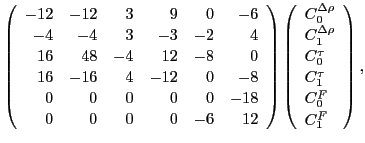
We recall here [23,29] that without the tensor terms, relations (62) and (63) allow us to determine the time-odd coupling constants $C_t^{s}$, $C_t^{\Delta s}$, and $C_t^{T}$ as functions of the time-even coupling constants $C_t^{\rho }$, $C_t^{\Delta \rho }$, and $C_t^{\tau }$. Since the time-even coupling constants are usually adjusted solely to the time-even observables, the resulting values of the time-odd coupling constants are simply ``fictitious'' or ``illusory'', as noted already in Ref. [30]. In a more realistic case of relations (49) and (50), these constraints are no longer valid, and the time-odd properties of the functional are independent of the time-even properties. This independence requires breaking the link between the Skyrme force and the density functional.