A new set of the ISB corrections to superallowed $\beta$-decays

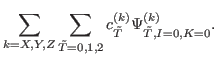
In this section we present results obtained within the NCCI model, which pertain to removing the uncertainty related to ambiguities in the shape-current orientation. Similar to our previous applications within the static model, the ground-states (g.s.) of even-even nuclei, $\vert I=0, T\approx 1, T_z = \pm 1 \rangle$, are approximated by the Coulomb $T$-mixed states,

$$\vert I=0, T\approx 1, T_z = \pm 1 \rangle = \Psi_{\tilde{T}=1,I=0,K=0}^{(1)}$$

$$= \sum_{T\geq 1} c^{(1)}_{T} \Psi_{T,I=0,K=0}^{(1)},$$ (1)

which were angular-momentum projected from the MF g.s. $\varphi_1$ of the even-even nuclei, obtained in the self-consistent Hartree-Fock (HF) calculations. States $\varphi_1$ are always unambiguously defined by filling in the pairwise doubly degenerate levels of protons and neutrons up to the Fermi level. In the calculations, the Coulomb $T$-mixing was included up to $T=4$.

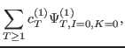
Within our dynamic model, the corresponding isobaric analogues in $N=Z$ odd-odd nuclei, $\vert I=0, T\approx 1, T_z = 0 \rangle$, were approximated by

$$\vert I=0, T\approx 1, T_z = 0 \rangle = \sum_{k=X,Y,Z} \sum_{\tilde{T}=0,1,2} c^{(k)}_{\tilde{T}} \Psi_{\tilde{T},I=0,K=0}^{(k)}.$$

The underlying MF states $\varphi_k$ were taken as the self-consistent Slater determinants $\vert\bar \nu \otimes \pi ; k \rangle$ (or $\vert \nu \otimes \bar \pi ; k \rangle$) representing the antialigned configurations corresponding to different shape-current orientations $k=X,Y,Z$. Let us recall that the antialigned states are constructed by placing the odd neutron and odd proton in the lowest available time-reversed (or signature-reversed) s.p. orbits. These states are manifestly breaking the isospin symmetry. Using them is the only way to reach the $\vert I=0, T\approx 1, T_z = 0 \rangle$ states in odd-odd $N=Z$ nuclei. The reason is that, within a conventional MF approach with separate proton and neutron Slater determinants, these states are not representable by single Slater determinants, see discussion in Ref. [21].

For odd-odd nuclei, mixing coefficients $c^{(k)}_{\tilde{T}}$ in Eq. (2) were determined by solving the Hill-Wheeler equation. In the mixing calculations, we only included states $\Psi_{\tilde{T},I=0,K=0}^{(k)}$ with dominating isospins of $\tilde{T}=0,1$ and 2, that is, the Hill-Wheeler equation was solved in the space of six or nine states for axial and triaxial states, respectively. We recall that each of states $\Psi_{\tilde{T},I=0,K=0}^{(k)}$ contains all Coulomb-mixed good-$T$ components $\Psi_{{T},I=0,K=0}^{(k)}$.

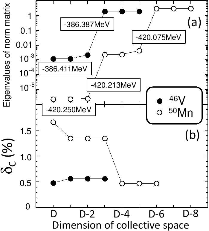
The three states corresponding to a given dominating isospin are linearly dependent. One may therefore argue that the physical subspace of the $I=0$ states should be three dimensional. In the calculations, all six or nine eigenvalues of the norm matrix ${\cal{N}}$ are nonzero, but the linear dependence of the reference states is clearly reflected in the pattern they form. For two representative examples of axial ($^{46}$V) and triaxial ($^{50}$Mn) nuclei, this is depicted in Fig. 2. Note, that the eigenvalues group into two or three sets, each consisting of three similar eigenvalues. Note also, that the differences between the sets are large, reaching three-four orders of magnitude. Lower part of the figure illustrates dependence of the calculated ISB corrections, $\delta _{\rm C}$, on a number of the collective states retained in the mixing. As shown, the calculated corrections are becoming stable within a subspace consisting five (or less) highest-norm states. Following this result, we have decided to retain in the mixing calculations only three collective states built upon the three eigenvectors of the norm matrix corresponding to the largest eigenvalues.

Figure 2: (a) Eigenvalues of the norm matrix obtained in the NCCI calculations for the $I=0$ states of odd-odd nuclei. Depicted are typical results obtained for two representative examples of axial ($^{46}$V) and triaxial ($^{50}$Mn) nuclei. The boxes give values of eigenenergies obtained by including three, six, or nine eigenvalues of the norm matrix. (b) Dependence of the ISB corrections to superallowed $^{46}$V $\rightarrow ^{46}$Ti and $^{50}$Mn $\rightarrow ^{50}$Cr decays on a number of collective states retained in the mixing calculations. Dimension of the collective space decreases from the left to the right hand side from $D$=9(6) in $^{50}$Mn($^{46}$V), respectively.

Based on this methodology, we calculated the set of the superallowed transitions, which are collected in Tables 1 and 2. Table 1 shows the empirical $ft$ values, calculated ISB corrections, and so-called nucleus-independent reduced lifetimes,

$${\cal F}t \equiv ft(1+\delta_{\rm R}^\prime)(1+\delta_{\rm NS} -\delta_{\rm C}) = \frac{K}{2 G_{\rm V}^2 (1 + \Delta^{\rm V}_{\rm R})},$$ (2)

where $\delta_{\rm R}^\prime$ and $\delta_{\rm NS}$ are the radiative corrections [27]. Errors of ${\cal F}t$ include errors of the empirical $ft$ values [28,29], radiative corrections $\delta_{\rm R}^\prime$ and $\delta_{\rm NS}$ [27], and our uncertainties estimated for the calculated values of $\delta _{\rm C}$.

Except for transitions $^{14}$O $\rightarrow$$^{14}$N and $^{42}$Sc $\rightarrow$$^{42}$Ca, all ISB corrections were calculated using the prescription sketched above. For the decay of a spherical nucleus $^{14}$O, the reference state is uniquely defined and thus the mixing of orientations was not necessary, whereas for that of $^{42}$Sc, an ambiguity of choosing its reference state is not related to the shape-current orientation. For both cases, the values and errors of $\delta _{\rm C}$ were taken from Ref. [15]. For the remaining cases, to account for uncertainties related to the basis size and collective-space cut-off, we assumed an error of 15%. This is larger than the 10% uncertainties related to the basis size only, which were assumed in Ref. [15].

Systematic errors related to the form and parametrization of the functional itself were not included in the error budget. Moreover, similarly to our previous works [14,15], transition $^{38}$K $\rightarrow$$^{38}$Ar was disregarded. We recall that for this transition, the calculated value of the ISB correction is unacceptably large because of a strong mixing of Nilsson levels originating from the $d_{3/2}$ and $s_{1/2}$ sub-shells. The problem can be partially cured by performing configuration-interaction calculations, see Ref. [18] and discussion in Sect. 4.2.

Table 1: Results of calculations performed for nuclei, for which the superallowed transitions have been measured. Listed are empirical $ft$ values [29]; calculated ISB corrections $\delta_{\rm C}^{{\rm (SV)}}$ and the corresponding ${\cal F}t$ values; empirical corrections $\delta_{\rm C}^{{\rm (exp)}}$ calculated using Eq. (5); contributions coming from the individual transitions to the $\chi^2$ budget in the confidence-level test. As in Ref. [29], we give two digits of the calculated errors of the ${\cal F}t$ values.

Parent	$ft$	$\quad$	$\delta_{\rm C}^{{\rm (SV)}}~\strut$	${\cal F}t~~~~~\strut$	$\quad$	$\delta_{\rm C}^{{\rm (exp)}}~\strut$	$\chi^2_i$
nucleus	(s)		(%)$~~~\strut$	(s) $~~~~~\strut$		(%)$~~~\strut$
$T_z=-1:$
$^{10}$C	3042(4)		0.579(87)	3064.5(52)		0.37(15)	3.5
$^{14}$O	3042.3(27)		0.303(30)	3072.3(33)		0.36(6)	0.0
$^{22}$Mg	3052(7)		0.270(41)	3081.4(72)		0.62(23)	1.4
$^{34}$Ar	3053(8)		0.87(13)	3063.6(91)		0.63(27)	1.3
$T_z=0:$
$^{26}$Al	3036.9(9)		0.329(49)	3071.8(20)		0.37(4)	0.8
$^{34}$Cl	3049.4(12)		0.75(11)	3067.6(38)		0.65(5)	10.9
$^{42}$Sc	3047.6(14)		0.77(27)	3069.2(85)		0.72(6)	3.1
$^{46}$V	3049.5(9)		0.563(84)	3075.1(32)		0.71(6)	1.3
$^{50}$Mn	3048.4(12)		0.476(71)	3076.5(32)		0.67(7)	2.4
$^{54}$Co	3050.8( $^{+11}_{-15}$)		0.586(88)	3075.6(36)		0.75(8)	1.3
$^{62}$Ga	3074.1(15)		0.78(12)	3093.1(48)		1.51(9)	43.2
$^{74}$Rb	3085(8)		1.63(24)	3078(12)		1.86(27)	0.3
			$\overline{{\cal F}t}=$	3073.7(11)		$\chi^2 =$	69.5
			$\vert V_{\rm ud}\vert=$	0.97396(25)		$\chi_d^2 =$	6.3
				0.99937(65)

Table 2: Similar as in Table 1 but for the transitions that are either unmeasured or measured with insufficient accuracy to be used for the SM tests.

Parent	$\delta_{\rm C}^{\rm (SV)}$	$\quad$	Parent	$\delta_{\rm C}^{\rm (SV)}$
nucleus			nucleus
	(%)			(%)
$T_z=-1:$			$T_z=0:$
$^{18}$Ne	1.37(21)		$^{18}$F	1.22(18)
$^{26}$Si	0.427(64)		$^{22}$Na	0.335(50)
$^{30}$S	1.24(19)		$^{30}$P	0.98(15)

To conform with the analyzes of Hardy and Towner (HT) and Particle Data Group, the average value $\overline{{\cal F}t} = 3073.7(11)$s was calculated using the Gaussian-distribution-weighted formula. This leads to the value of $\vert V_{\rm ud}\vert = 0.97396(25)$, which is in a very good agreement both with the Hardy and Towner result [29], $\vert V_{\rm ud}^{{\rm (HT)}}\vert = 0.97425(22)$, and central value obtained from the neutron decay $\vert V_{\rm ud}^{(\nu )}\vert = 0.9746(19)$ [30]. By combining the value of $\vert V_{\rm ud}\vert$ calculated here with those of $\vert V_{\rm us}\vert = 0.2253(8)$ and $\vert V_{\rm ub}\vert = 0.00413(49)$ of the 2014 Particle Data Group [3], one obtains

$$\vert V_{\rm ud}\vert^2 + \vert V_{\rm us}\vert^2 + \vert V_{\rm ub}\vert^2 = 0.99937(65),$$ (3)

which implies that the unitarity of the first row of the CKM matrix is satisfied with a precision better than 0.1%. Note that, in spite of differences between individual values of $\delta _{\rm C}$, the values of $\overline{{\cal F}t}$ and $\vert V_{\rm ud}\vert$ obtained here are in excellent agreement with the results of our previous works [14,15].

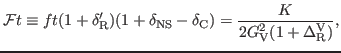
The last two columns of Table 1 show results of the confidence-level (CL) test, as proposed in Ref. [28]. The CL test is based on the assumption that the CVC hypothesis is valid up to at least $\pm 0.03$%, which implies that a set of structure-dependent corrections should produce statistically consistent set of ${\cal F}t$-values. 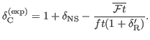Assuming the validity of the calculated corrections $\delta_{\rm NS}$ [31], the empirical ISB corrections can be defined as:

$$\delta_{\rm C}^{{\rm (exp)}} = 1 + \delta_{\rm NS} - \frac{\overline{{\cal F}t}}{ft(1+\delta_{\rm R}^\prime)}.$$ (4)

By the least-square minimization of the appropriate $\chi^2$, and treating the value of $\overline{{\cal F}t}$ as a single adjustable parameter, one can attempt to bring the set of empirical values $\delta_{\rm C}^{{\rm (exp)}}$ as close as possible to the set of $\delta _{\rm C}$.

The empirical ISB corrections deduced in this way are tabulated in Table 1. The table also lists individual contributions to the $\chi^2$ budget, whereas the total $\chi^2$ per degree of freedom ( $\chi_d^2=\chi^2/n_d$ for $n_d=11$) is $\chi_d^2 = 6.3$. This number is considerably smaller than the number quoted in our previous work [15], but much bigger than those obtained within (i) perturbative-model reported in Ref. [28] (1.5), (ii) shell model with the Woods-Saxon radial wave functions (0.4) [27], (iii) shell model with Hartree-Fock radial wave functions (2.0) [32,33], (iv) Skyrme-Hartree-Fock with RPA (2.1) [34], and relativistic Hartree-Fock plus RPA model (1.7) [35]. It is worth stressing that, as before, our value of $\chi^2 /n_d$ is deteriorated by two transitions that strongly violate the CVC hypothesis, $^{62}$Ga $\rightarrow ^{62}$As and $^{34}$Cl $\rightarrow ^{34}$S. These transitions give the 62% and 15% contributions to the total error budget, respectively. Without them, we would have obtained $\chi_d^2 = \chi^2 /9 = 1.7$.