Next: A=62 nuclei: Zn and Up: Low-energy spectra of selected Previous: states in Ca, K,
Within the conventional shell model, the ![]() Ca and
Ca and ![]() Sc nuclei
are treated as two-body systems above the core of
Sc nuclei
are treated as two-body systems above the core of ![]() Ca. Hence,
they are often used by the shell-model community to adjust the
isoscalar
Ca. Hence,
they are often used by the shell-model community to adjust the
isoscalar ![]() =0;
=0;![]() =1, 3, 5, 7, and isovector
=1, 3, 5, 7, and isovector ![]() =1;
=1;![]() =0, 2, 4, 6
matrix elements within the
=0, 2, 4, 6
matrix elements within the ![]() shell. Here, we use these
nuclei to test our NCCI model but, at least at this stage, without an
intention of refitting the interaction. The aim of this exercise is to
capture global trends and tendencies, which may allow us to identify
systematic features of the NCCI model in describing these
seemingly simple nuclei. From the perspective of our approach, such
tests are by no means trivial, because these nuclei are here treated within
the full core-polarization effects included, cf. discussion in
Refs. [53,54].
shell. Here, we use these
nuclei to test our NCCI model but, at least at this stage, without an
intention of refitting the interaction. The aim of this exercise is to
capture global trends and tendencies, which may allow us to identify
systematic features of the NCCI model in describing these
seemingly simple nuclei. From the perspective of our approach, such
tests are by no means trivial, because these nuclei are here treated within
the full core-polarization effects included, cf. discussion in
Refs. [53,54].
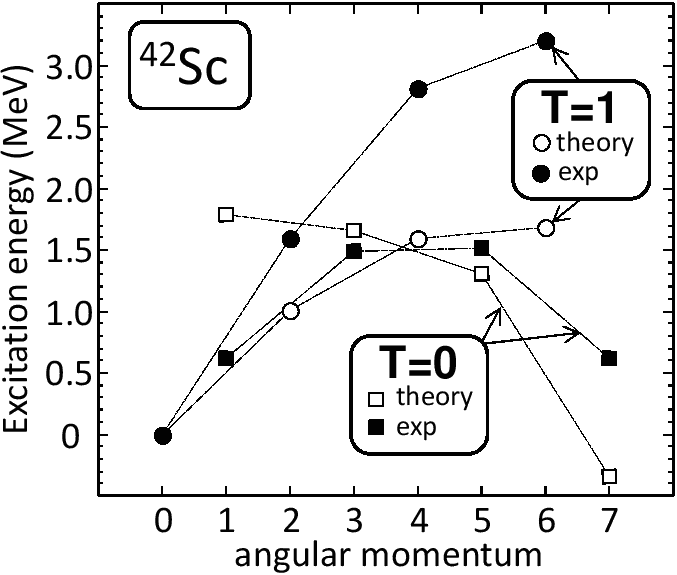
The results of the NCCI calculations for the isovector and isoscalar
multiplets in ![]() nuclei are depicted in Figs. 5
and 6, and collected in Table 5. The
reference states used in the calculation for
nuclei are depicted in Figs. 5
and 6, and collected in Table 5. The
reference states used in the calculation for ![]() Sc are listed in
Table 6. They cover all fully aligned (
Sc are listed in
Table 6. They cover all fully aligned (
![]() )
states, which are almost purely isoscalar, all possible
antialigned states (
)
states, which are almost purely isoscalar, all possible
antialigned states (
![]() ), and two
), and two ![]() aligned states.
The antialigned states manifestly violate the isospin symmetry and,
as discussed in Ref. [55], are approximately fifty-fifty
mixtures of the isoscalar and isovector components. The
aligned states.
The antialigned states manifestly violate the isospin symmetry and,
as discussed in Ref. [55], are approximately fifty-fifty
mixtures of the isoscalar and isovector components. The ![]() aligned
states also violate the isospin symmetry.
aligned
states also violate the isospin symmetry.
 |
|
|
|||||
| 0 |
|||||
| 2 |
1.012 | 1.586 | 1.357 | 1.525 | |
| 4 |
1.590 | 2.815 | 2.005 | 2.752 | |
| 6 |
1.696 | (3.200) | 2.154 | 3.189 | |
| 1 |
1.785 | 0.611 | |||
| 3 |
1.656 | 1.490 | |||
| 5 |
1.336 | 1.510 | |||
| 7 |
0.617 |
The following three general conclusions can be drown from the results presented in Fig. 5:
| 1 |
|
0.000 | 0.063 | 0 | 0.000 |
| 2 |
|
0.802 | 0.031 | 0 | 0.561 |
| 3 |
|
0.986 | 0.008 | 60 | 0.551 |
| 4 |
|
0.759 | 0.062 | 60 | 0.085 |
| 5 |
|
0.061 | 60 | -0.647 | |
| 6 |
|
0.082 | 0.007 | 60 | 1.160 |
| 7 |
|
0.345 | 0.032 | 0 | 1.594 |
| 8 |
|
0.340 | 0.060 | 0 | 1.719 |
| 9 |
|
0.716 | 0.043 | 0 | 2.164 |
| 10 |
|
0.986 | 0.011 | 0 | 2.338 |
In the case of ![]() Ca, we focused on calculating the excitation
energies of the
Ca, we focused on calculating the excitation
energies of the ![]() states, addressing, in particular, the question
of structure and excitation energy of the intruder
configuration. Experimentally, the intruder configuration is observed
at very low excitation energy of 1.843MeV, see Ref. [56]
and references cited therein. In the calculations presented below we
assumed that the structure of intruder state is associated with
(multi)particle-(multi)hole excitations across the
states, addressing, in particular, the question
of structure and excitation energy of the intruder
configuration. Experimentally, the intruder configuration is observed
at very low excitation energy of 1.843MeV, see Ref. [56]
and references cited therein. In the calculations presented below we
assumed that the structure of intruder state is associated with
(multi)particle-(multi)hole excitations across the ![]() magic gap,
which in
magic gap,
which in ![]() Ca is of the order of 7.0MeV, see Ref. [53]
and references cited therein. The mechanism bringing the intruder
configuration down in energy is sketched in
Fig. 7.
Ca is of the order of 7.0MeV, see Ref. [53]
and references cited therein. The mechanism bringing the intruder
configuration down in energy is sketched in
Fig. 7.
The energy needed to elevate particles from the ![]() subshell to
subshell to
![]() is at (near)spherical shape reduced by the energy
associated with the spontaneous breaking of spherical symmetry in the
intruder configuration, and further, by a rotational correction
energy associated with the symmetry restoration. Owing to the
configuration interaction, an additional gain in energy is expected
too. The rotational correction and configuration interaction are also
expected to lower slightly the MF g.s. energy. As shown in
Fig. 7, the final value of the intruder excitation
energy is an effect of rather a delicate interplay of several
factors. Therefore, it is not surprising that the intruder states
pose a real challenge for both the state-of-the-art nuclear shell
models and MF-rooted theories.
is at (near)spherical shape reduced by the energy
associated with the spontaneous breaking of spherical symmetry in the
intruder configuration, and further, by a rotational correction
energy associated with the symmetry restoration. Owing to the
configuration interaction, an additional gain in energy is expected
too. The rotational correction and configuration interaction are also
expected to lower slightly the MF g.s. energy. As shown in
Fig. 7, the final value of the intruder excitation
energy is an effect of rather a delicate interplay of several
factors. Therefore, it is not surprising that the intruder states
pose a real challenge for both the state-of-the-art nuclear shell
models and MF-rooted theories.
 |
In the NCCI calculations presented below, we mix states projected
from the antialigned configurations that are listed in
Table 7. The reference states can be divided into two
classes. The first four configurations do not involve any
cross-shell excitations. They correspond to the
![]() 0p-0h
0p-0h
![]() configurations with
magnetic quantum number of
configurations with
magnetic quantum number of ![]() =1/2, 3/2, 5/2, and 7/2, respectively. The
three remaining configurations are the lowest MF configurations
involving two
=1/2, 3/2, 5/2, and 7/2, respectively. The
three remaining configurations are the lowest MF configurations
involving two
![]() , four
, four
![]() , and six
, and six
![]() holes in
holes in ![]() shell, respectively.
shell, respectively.
| 1 |
|
0.000 | 0.069 | 0 |
0.000 |
| 2 |
|
0.516 | 0.033 | 0 |
0.765 |
| 3 |
|
0.544 | 0.007 | 60 |
0.770 |
| 4 |
|
0.084 | 0.061 | 60 |
0.315 |
| 5 |
|
10.001 | 0.288 | 14 |
6.860 |
| 6 |
|
10.986 | 0.414 | 22 |
6.498 |
| 7 |
|
14.937 | 0.542 | 12 |
9.619 |
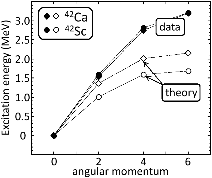
The results of the NCCI calculations in ![]() Ca are depicted in
Figs. 6 and 8 and collected in
Tables 5 and 7. Figure 6 shows the
Ca are depicted in
Figs. 6 and 8 and collected in
Tables 5 and 7. Figure 6 shows the
![]() , and 6
, and 6![]() states - the isovector
states - the isovector ![]() =1 multiplet -
obtained within the NCCI calculations involving only
=1 multiplet -
obtained within the NCCI calculations involving only
![]() reference states. The results are qualitatively similar to those in
reference states. The results are qualitatively similar to those in
![]() Sc. In both cases, theoretical spectra are compressed as
compared to data. Detailed quantitative comparison reveals, however,
surprisingly large differences between the theoretical and experimental
spectra.
Sc. In both cases, theoretical spectra are compressed as
compared to data. Detailed quantitative comparison reveals, however,
surprisingly large differences between the theoretical and experimental
spectra.
First, the energy differences
![]() for
for
![]() are positive (negative) in theory (experiment), respectively. Second,
the absolute values of
are positive (negative) in theory (experiment), respectively. Second,
the absolute values of
![]() are a few times larger in
theory as compared to the data. It means that the model tends to
overestimate the ISB effects in clearly an unphysical manner. This
influences the ISB correction to the
are a few times larger in
theory as compared to the data. It means that the model tends to
overestimate the ISB effects in clearly an unphysical manner. This
influences the ISB correction to the
![]() Fermi
Fermi
![]() -decay matrix element, which in the present NCCI calculation
rises to
-decay matrix element, which in the present NCCI calculation
rises to
![]() %. Most likely, the unphysical
component in the ISB effect is related to the time-odd polarizations and
matrix elements originating from these fields, which are essentially
absent in even-even systems. One should also remember that in the
Skyrme functionals, including, of course, the SV force used here, the
time-odd terms are very purely constrained.
%. Most likely, the unphysical
component in the ISB effect is related to the time-odd polarizations and
matrix elements originating from these fields, which are essentially
absent in even-even systems. One should also remember that in the
Skyrme functionals, including, of course, the SV force used here, the
time-odd terms are very purely constrained.
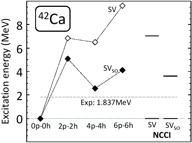 |
Figure 8 shows the ![]() states calculated using
functionals SV. The left part of the figure depicts the
lowest
states calculated using
functionals SV. The left part of the figure depicts the
lowest ![]() states projected from the reference states
states projected from the reference states
![]() (0p-0h),
(0p-0h),
![]() (2p-2h),
(2p-2h),
![]() (4p-4h), and
(4p-4h), and
![]() (6p-6h).
These results do not include configuration mixing. Note, that
symmetry restoration itself changes the optimal intruder
configuration to
(6p-6h).
These results do not include configuration mixing. Note, that
symmetry restoration itself changes the optimal intruder
configuration to
![]() as compared to MF, which
favors
as compared to MF, which
favors
![]() .
.
The right part of the figure shows excitation energies of the
intruder states as obtained within the NCCI calculations. Here, all
reference states listed in Table 7 were included. For the
SV force, the excitation energy of the lowest intruder configuration
equals 7.5MeV, and exceeds the data by 5.7MeV. The main reason of
the disagreement is related to an unphysically large ![]() shell
gap: the bare
shell
gap: the bare ![]() gap deduced directly from the s.p. HF levels in
gap deduced directly from the s.p. HF levels in
![]() Ca equals as much as 11.5MeV. Its value exceeds the
experimental gap by almost 4.5MeV (for an overview of experimental
data, see Ref. [53] and references cited therein). It is
therefore not surprising that the combined effects of deformation and
rotational correction are unable to compensate for the large energy
needed to lift the particles from the
Ca equals as much as 11.5MeV. Its value exceeds the
experimental gap by almost 4.5MeV (for an overview of experimental
data, see Ref. [53] and references cited therein). It is
therefore not surprising that the combined effects of deformation and
rotational correction are unable to compensate for the large energy
needed to lift the particles from the ![]() to
to ![]() shell,
see Fig. 7.
shell,
see Fig. 7.
To investigate interplay between the s.p. and collective
effects, we repeated the NCCI calculations using the functional
SV![]() , which differs from SV in a single aspect, namely, we
increased its spin-orbit strength by a factor of 1.2. This readjustment allows to reduce
a disagreement between theoretical and experimental binding energies in
, which differs from SV in a single aspect, namely, we
increased its spin-orbit strength by a factor of 1.2. This readjustment allows to reduce
a disagreement between theoretical and experimental binding energies in
![]()
![]() and lower-
and lower-![]() shell nuclei to
shell nuclei to ![]() 1% level as shown in Ref. [57].
When applied to the heaviest
1% level as shown in Ref. [57].
When applied to the heaviest ![]() nucleus
nucleus ![]() Sn and its neighbor
Sn and its neighbor ![]() In it gives
827.710 MeV and 833.067 MeV what is in an impressive agreement with the experimental binding energies
equal 825.300 MeV (833.110 MeV) in
In it gives
827.710 MeV and 833.067 MeV what is in an impressive agreement with the experimental binding energies
equal 825.300 MeV (833.110 MeV) in ![]() Sn (
Sn (![]() In), respectively.
Ability to reproduce masses is among the most important indicators of a quality of DFT-based models.
Such a readjustment of the SO strength is also the simplest
and most efficient mechanism allowing us to reduce the magic
In), respectively.
Ability to reproduce masses is among the most important indicators of a quality of DFT-based models.
Such a readjustment of the SO strength is also the simplest
and most efficient mechanism allowing us to reduce the magic ![]() gap [58]. For the SV
gap [58]. For the SV![]() force, the bare gap equals
9.6MeV, which is by almost 1.9MeV smaller than the original SV
gap, but still it is much larger, by circa 2.6MeV, than the
experimental value. Results of the NCCI calculations obtained using
functional SV
force, the bare gap equals
9.6MeV, which is by almost 1.9MeV smaller than the original SV
gap, but still it is much larger, by circa 2.6MeV, than the
experimental value. Results of the NCCI calculations obtained using
functional SV![]() are shown in Fig. 8. Now the
projected and NCCI calculations both favor the configuration
are shown in Fig. 8. Now the
projected and NCCI calculations both favor the configuration
![]() . We also note that for both the SV and SV
. We also note that for both the SV and SV![]() functionals, geometrical properties of the reference states
(deformations) are very similar.
functionals, geometrical properties of the reference states
(deformations) are very similar.
When discussing the influence of various effects on the final
position of the intruder state, it is worth stressing the role of the
symmetry restoration. The rotational correction lowers the intruder
state by 4.9MeV, bringing its excitation energy to 2.3MeV, which
is only 0.5MeV above the experiment. However, after the
configuration mixing, the excitation energy of the intruder state
increases to about 3.6MeV, that is, it becomes again 1.7MeV
higher as compared to data. This is due to the configuration mixing
in the ground state, which lowers its energy by almost 1MeV,
whereas it leaves the position of the intruder state almost
unaffected. The reason for that is the fact that the
![]() antialigned reference states (states 1-4 in
Tables 7 and 8) are almost linearly
dependent and thus mix relatively
strongly. Conversely, at deformations corresponding to the intruder
configuration
antialigned reference states (states 1-4 in
Tables 7 and 8) are almost linearly
dependent and thus mix relatively
strongly. Conversely, at deformations corresponding to the intruder
configuration
![]() , the Nilsson scheme prevails.
Therefore, the intruder configurations become almost linearly
independent and appear to mix very weakly. The amount of the mixing
was tested by performing additional calculations of matrix elements
between the lowest
, the Nilsson scheme prevails.
Therefore, the intruder configurations become almost linearly
independent and appear to mix very weakly. The amount of the mixing
was tested by performing additional calculations of matrix elements
between the lowest
![]() configuration and the
excited configurations involving the same number of
configuration and the
excited configurations involving the same number of
![]() holes. All these matrix elements turned out to be negligibly small.
holes. All these matrix elements turned out to be negligibly small.
| 1 |
|
0.000 | 0.064 | 0 |
0.000 |
| 2 |
|
0.517 | 0.032 | 0 |
0.679 |
| 3 |
|
0.496 | 0.007 | 60 |
0.676 |
| 4 |
|
0.006 | 0.061 | 60 |
0.200 |
| 5 |
|
8.399 | 0.276 | 15 |
5.085 |
| 6 |
|
7.377 | 0.402 | 22 |
2.548 |
| 7 |
|
9.955 | 0.532 | 15 |
4.103 |
Jacek Dobaczewski 2016-03-05
