Next: Summary and perspectives Up: Low-energy spectra of selected Previous: A=42 nuclei: Sc and
For ![]() Zn, the results of the NCCI calculations of the low-lying
Zn, the results of the NCCI calculations of the low-lying
![]() states were communicated in Ref. [18]. Here, for the
sake of completeness, we briefly summarize the
results obtained therein. The calculated spectrum of the
states were communicated in Ref. [18]. Here, for the
sake of completeness, we briefly summarize the
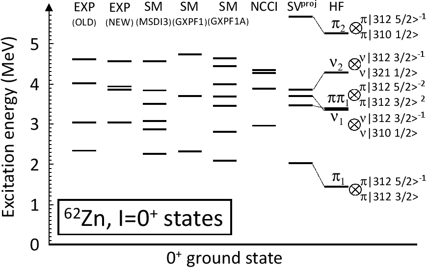
results obtained therein. The calculated spectrum of the ![]() states
below the excitation energy of 5MeV is shown in Fig. 9.
The NCCI calculations were based on six reference states that include:
the ground state, the two lowest neutron p-h excitations
states
below the excitation energy of 5MeV is shown in Fig. 9.
The NCCI calculations were based on six reference states that include:
the ground state, the two lowest neutron p-h excitations ![]() and
and
![]() , the two lowest proton p-h excitations
, the two lowest proton p-h excitations ![]() and
and ![]() ,
and the lowest proton 2p-2h excitation
,
and the lowest proton 2p-2h excitation ![]() . Their properties
are listed in Table 9.
. Their properties
are listed in Table 9.
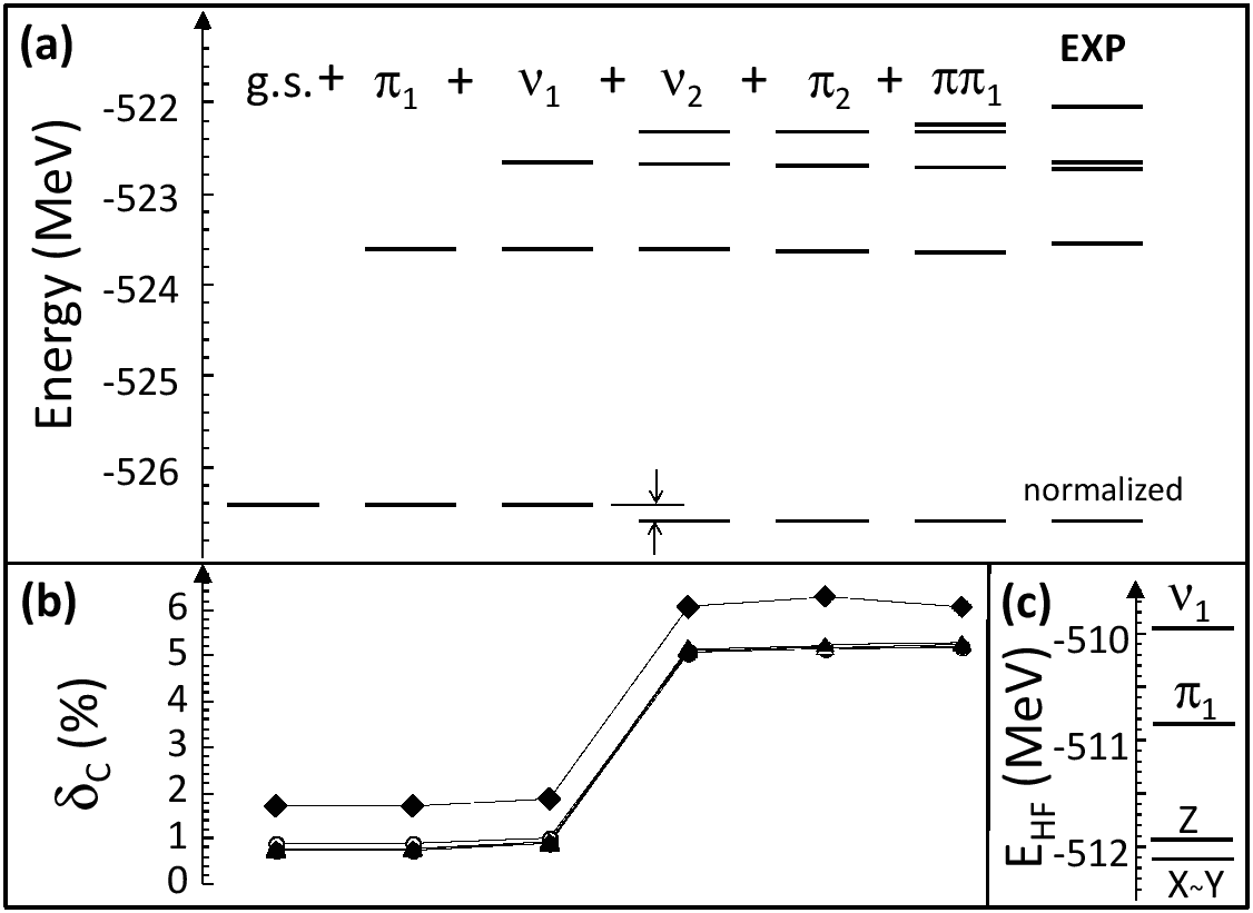
As discussed in Ref. [18], the calculated spectrum of
![]() states is in a very good agreement with the recent data
communicated by Leach et al. [59]. As shown in
Fig. 10(a), the calculated total g.s. energy is stable
with increasing the number of reference configurations. Its value of
states is in a very good agreement with the recent data
communicated by Leach et al. [59]. As shown in
Fig. 10(a), the calculated total g.s. energy is stable
with increasing the number of reference configurations. Its value of
![]() 526.595MeV (
526.595MeV (![]() harmonic oscillator shells were used)
underestimates the experiment by roughly 2%.
harmonic oscillator shells were used)
underestimates the experiment by roughly 2%.
| 1 | g.s. | 0.270 | 31 |
0.000 | 0.000 | |||
| 2 | 1.433 | 0.286 | 20 |
0.005 | 0.152 | Y | 2.036 | |
| 3 | 3.347 | 0.255 | 40 |
0.689 | 0.318 | X | 3.703 | |
| 4 | 4.287 | 0.240 | 25 |
Y | 3.852 | |||
| 5 | 5.251 | 0.246 | 48 |
X | 5.672 | |||
| 6 | 3.381 | 0.251 | 38 |
0.000 | 0.000 | 3.471 |
| 1 | Y | 0.268 | 30 |
0.149 | Y | |||
| 2 | X | 0.007 | 0.268 | 30 |
0.180 | X | ||
| 3 | Z | 0.190 | 0.269 | 30 |
0.264 | Z | 0.005 | |
| 4 | 1.266 | 0.284 | 20 |
X | 2.175 | |||
| 5 | 1.977 | 0.255 | 35 |
X | 3.151 |
 |
In spite of the fact that the total binding energy is relatively
stable, the calculated ISB corrections to superallowed transition
![]() Ga
Ga
![]() Zn strongly depend on the details of the
calculation. This is illustrated in Fig.10(b), which
shows values of
Zn strongly depend on the details of the
calculation. This is illustrated in Fig.10(b), which
shows values of
![]() in function of the number of
configurations taken for the NCCI calculations in the daughter
nucleus
in function of the number of
configurations taken for the NCCI calculations in the daughter
nucleus ![]() Zn. The four different curves correspond to different
model spaces taken for the NCCI calculation in the parent nucleus
Zn. The four different curves correspond to different
model spaces taken for the NCCI calculation in the parent nucleus
![]() Ga, see Table 10 and Fig. 10(c).
In terms of Nilsson numbers, counted relatively to the
Ga, see Table 10 and Fig. 10(c).
In terms of Nilsson numbers, counted relatively to the ![]() Zn
Zn![]() even-even
core, the configurations X,Y,Z correspond to differently aligned
even-even
core, the configurations X,Y,Z correspond to differently aligned
![]() two-hole states,
two-hole states, ![]() denotes
denotes
![]() ,
two hole state while
,
two hole state while ![]() is
is
![]() .
The three curves labeled with open dots, and open and filled triangles
correspond to states
.
The three curves labeled with open dots, and open and filled triangles
correspond to states ![]() projected from the [X,Y], [X,Y,Z], and
[X,Y,Z,
projected from the [X,Y], [X,Y,Z], and
[X,Y,Z,![]() ] configurations, respectively. These curves
essentially overlap with each other, thus showing no influence of the
configuration-mixing (in this restricted model space) on the
structure of the
] configurations, respectively. These curves
essentially overlap with each other, thus showing no influence of the
configuration-mixing (in this restricted model space) on the
structure of the ![]() state in the parent nucleus. Note, however,
that an extension of the model space by adding the lowest neutron p-h
excitation, [X,Y,Z,
state in the parent nucleus. Note, however,
that an extension of the model space by adding the lowest neutron p-h
excitation, [X,Y,Z,![]() ,
,![]() ], leads to an increase in
], leads to an increase in
![]() of about 1%. Note also, that all curves are
particularly sensitive to an admixture of the
of about 1%. Note also, that all curves are
particularly sensitive to an admixture of the ![]() configuration
in the daughter nucleus. This admixture increases
configuration
in the daughter nucleus. This admixture increases
![]() by
almost 4%. The analysis clearly shows that, within the present
implementation of the model, it is essentially impossible to match
the spaces of states used to calculate the parent and daughter
nuclei. The reasons are manifold. The lack of representability of the
by
almost 4%. The analysis clearly shows that, within the present
implementation of the model, it is essentially impossible to match
the spaces of states used to calculate the parent and daughter
nuclei. The reasons are manifold. The lack of representability of the
![]() states in the
states in the ![]() nucleus within the conventional MF using
products of neutron and proton wave functions and difficulties in
constraining the time-odd part of the functional are two of them.
Difficulty of matching the model spaces in the parent and daughter
nuclei introduce here an artificial ISB effect. As a result, beyond a
simple mixing of orientations used in the result given in
Table 1, the NCCI approach cannot be used for
determining the ISB corrections to the transition
nucleus within the conventional MF using
products of neutron and proton wave functions and difficulties in
constraining the time-odd part of the functional are two of them.
Difficulty of matching the model spaces in the parent and daughter
nuclei introduce here an artificial ISB effect. As a result, beyond a
simple mixing of orientations used in the result given in
Table 1, the NCCI approach cannot be used for
determining the ISB corrections to the transition
![]() Ga
Ga
![]() Zn.
Zn.
 |
Jacek Dobaczewski 2016-03-05