Since pairing is neglected in this work, the charge quadrupole moments
![]() and
and
![]() are defined microscopically as sums of
expectation values of the s.p. quadrupole moment operators
and
are defined microscopically as sums of
expectation values of the s.p. quadrupole moment operators
and  of the occupied proton states, i.e.,
are defined in three-dimensional
Cartesian coordinates as [22] (conserved signature symmetry is assumed)
 |
(3) | ||
| (4) |
in order to have the following expressions for the total quadrupole moment
Note that the sums in Eqs. (1-2) run only over proton states. The neutrons, having zero electric charge, do not appear in the sums explicitly, but they influence the charge quadrupole moments indirectly via the quadrupole polarization (deformation changes) induced by occupying/emptying single-neutron states.
It should be noted that with the definitions (1-6),
the spherical components of the quadrupole tensor are ![]() and
and
![]() . This fact is important for the definition of the
so-called transition quadrupole moment
. This fact is important for the definition of the
so-called transition quadrupole moment ![]() [23,24].
This moment gives the measure of the transition strength of the
[23,24].
This moment gives the measure of the transition strength of the
![]() =2 (stretched)
=2 (stretched)
![]() radiation in the limit of large deformation and angular momentum, and it is
proportional to the component
radiation in the limit of large deformation and angular momentum, and it is
proportional to the component
![]() of the
spherical quadrupole tensor when the quantization axis coincides with
the vector of rotational velocity
of the
spherical quadrupole tensor when the quantization axis coincides with
the vector of rotational velocity ![]() , i.e.,
, i.e.,
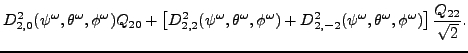
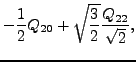
| (7) | |||
![$\displaystyle D^2_{2, 0}(\psi^{\omega},\theta^{\omega},\phi^{\omega})Q_{20}
+ \...
...2}(\psi^{\omega},\theta^{\omega},\phi^{\omega})\right]
\frac{Q_{22}}{\sqrt{2}}.$](img69.png) |
(8) |
 being
the Euler angles that rotate the
being
the Euler angles that rotate the
For the cranking axis coinciding with the ![]() -axis of the intrinsic
system, as is the case for the code HFODD [26,27] used
in the present study, the Euler angles are
-axis of the intrinsic
system, as is the case for the code HFODD [26,27] used
in the present study, the Euler angles are ![]() =0,
=0, ![]() =
=![]() ,
and
,
and ![]() =
=![]() , which gives:
, which gives:
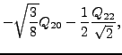
| (9) | |||
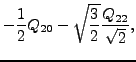 |
(10) |
In order to provide a link to studies that employ
the 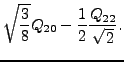 -axis cranking, like, e.g.,
Refs. [23,24]
and our earlier papers [21,20], we repeat
derivations for the Euler angles
-axis cranking, like, e.g.,
Refs. [23,24]
and our earlier papers [21,20], we repeat
derivations for the Euler angles
![]() =
=![]() ,
, ![]() =
=![]() ,
, ![]() =
=![]() , which rotate the
, which rotate the ![]() axis
onto the axis:
axis
onto the axis:
| (12) | |||
 |
(13) |
Although definitions (11) and (14) differ by signs
of the second terms, values of
 and
and
![]() obtained in self-consistent
calculations must be identical because they cannot
depend on the direction of the cranking axis. It means that
values of
obtained in self-consistent
calculations must be identical because they cannot
depend on the direction of the cranking axis. It means that
values of ![]() obtained in cranking calculations along the
obtained in cranking calculations along the ![]() and axes have opposite signs. In what follows,
we employ definition (11) of the transition moment
and drop the superscripts that denote the direction of the
cranking axis, e.g.,
and axes have opposite signs. In what follows,
we employ definition (11) of the transition moment
and drop the superscripts that denote the direction of the
cranking axis, e.g.,
Finally, the expectation value of the total angular momentum
![]() (its projection
on the cranking axis) is defined as a sum
of the expectation values of the s.p. angular momentum operators
(its projection
on the cranking axis) is defined as a sum
of the expectation values of the s.p. angular momentum operators
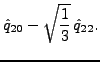 of the occupied states
| (17) |
 |
(18) |