Solution of the Hartree-Fock-Bogolyubov equations

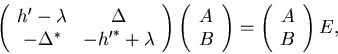
In order to incorporate pairing correlations for rotating states, the new version (v2.07f) of the code HFODD solves the standard HFB equation [10],

$$\left(\begin{array}{cc} h' - \lambda & \Delta \\ -\Delta^... ...right) = \left(\begin{array}{c} A \\ B \end{array}\right) E ,$$ (6)

by using the Cartesian HO basis. Here, $h'$ is the s.p. Routhian operator (I-26), with the cranking term $-\mbox{{\boldmath {$\omega$}}}\cdot\hat{\mbox{{\boldmath {$J$}}}}_0$ generalized to three dimensions, $\lambda$ is the Fermi energy (the HFB equation is solved separately for protons and neutrons), $\Delta$ is the antisymmetric pairing potential, $E$ is a diagonal matrix of quasiparticle energies, and $A$ and $B$ are the upper and lower components of the quasiparticle wavefunctions.

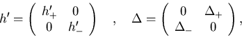
For the conserved simplex symmetry, which in the present version is assumed when solving the HFB equation, the Routhian and the pairing potential acquire the following block forms [12,10]:

$$h' = \left(\begin{array}{cc} h'_{+} & 0 \\ 0& h'_{-}\end... ...y}{cc} 0 & \Delta_{+} \\ \Delta_{-} & 0 \end{array}\right) ,$$ (7)

where the first and second halfs of the basis states correspond to positive and negative simplex, respectively. Therefore, the HFB equation decouples into two independent equations, of which only one needs to be solved. The code HFODD solves the equation

$$\left(\begin{array}{cc} h'_{+}-\lambda & \Delta_{+} \\ -\... ...\begin{array}{cc} E_{-} & 0 \\ 0 & -E_{+}\end{array}\right),$$ (8)

from which the complete solution of Eq. (6) is reconstructed as

$$A = \left(\begin{array}{cc} 0 & A_{+} \\ A_{-} & 0 \end{... ...(\begin{array}{cc} E_{+} & 0 \\ 0& E_{-}\end{array}\right) .$$ (9)

Note that if the s.p. space contains $M$ states ($M$/2 in each of the two simplexes $s$=$\pm{i}$), then the HFB equation (6) has a dimension of $2M$$\times$$2M$, matrices without the $\pm$ indices ($h'$, $\Delta$, $A$, $B$, ...) have a dimension of $M$$\times$$M$, and matrices with the $\pm$ indices ($h'_\pm$, $\Delta_\pm$, $A_\pm$, $B_\pm$, ...) have a dimension of $M/2$$\times$$M/2$. Hence, equation (8), which the code solves, has the dimension $M$$\times$$M$ which is twice smaller than the complete HFB equation (6). Note also that we use the convention of indices $\pm$ such that they correspond to simplexes of the left matrix indices.

For the conserved time-reversal symmetry, diagonal matrices of eigenvalues $E_{+}$ and $E_{-}$ are identical to one another, and the separation of eigenvectors of Eq. (8) into two simplexes is trivial; it is enough to group positive and negative quasiparticle energies together. For broken time-reversal this procedure does not work, because there can be more than half positive or negative quasiparticle energies in the spectrum of Eq. (8). So in general one has to put the half of largest eigenvalues into matrix $E_{-}$, and the half of smallest into matrix $E_{+}$, irrespective of their signs. Such a choice leads to the solution that corresponds to the so-called quasiparticle vacuum.

Based on the solution of the matrix equation (8), we have upper and lower components of the quasiparticle wave functions in the space coordinates as 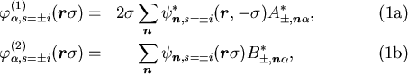where $\psi_{{\mbox{{\boldmath {${\scriptstyle n}$}}}},s=\pm{i}}(\mbox{{\boldmath {$r$}}}\sigma)$ are the HO simplex wave functions (I-78) in space coordinates (I-76) and $\mbox{{\boldmath {$n$}}}$=$(n_x,n_y,n_z)$ are the numbers of the HO quanta in three Cartesian directions. In Eq. (10) we have used the fact that the s.p. basis states of either of the two simplexes, $s=\pm{i}$, can be numbered by the HO quantum numbers $\mbox{{\boldmath {$n$}}}$. We have also introduced index $\alpha$=1,...,$M/2$, which numbers eigenstates of Eq. (8) in both "halfs" of the spectrum defined above.

From the quasiparticle wave functions we obtain the standard particle and pairing density matrices [13], 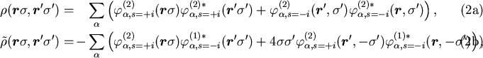where the sum over $\alpha$ is performed up to the maximum equivalent-spectrum energy $\bar{e}_{\mbox{\scriptsize {max}}}$, see Ref. [14] for details. All particle-hole mean-field potentials can be calculated from the particle density matrix $\rho (\mbox{{\boldmath {$r$}}}\sigma,\mbox{{\boldmath {$r$}}}'\sigma')$ and its derivatives (see I), while the particle-particle mean-field potentials can be calculated from the pairing density matrix $\tilde{\rho}(\mbox{{\boldmath {$r$}}}\sigma,\mbox{{\boldmath {$r$}}}'\sigma')$ [13]. In the present implementation of the code HFODD, terms depending on derivatives of the particle-particle density matrix are not taken into account, and hence the pairing potential depends only on the local pair density

$$\tilde{\rho}(\mbox{{\boldmath {$r$}}}) = -2\sum_{\alpha\sigm... ...arphi^{(1)*}_{\alpha,s=-{i}}(\mbox{{\boldmath {$r$}}}\sigma) ,$$ (10)

i.e.,

$$\tilde{h}(\mbox{{\boldmath {$r$}}}) = {\textstyle{\frac{1}{2... ...ox{{\boldmath {$r$}}})\tilde{\rho}(\mbox{{\boldmath {$r$}}}) ,$$ (11)

where $f(\mbox{{\boldmath {$r$}}})$ is the standard formfactor of the zero-range density-dependent pairing force,

$$f(\mbox{{\boldmath {$r$}}}) = V_0 + V_1\rho^\alpha(\mbox{{\b... ...ho(\mbox{{\boldmath {$r$}}})}{\rho_0} \right)^\alpha\right) .$$ (12)

Note that an attractive interaction requires $V_0$$<$0.

Finally, matrix elements of the pairing potential in the simplex HO basis, which are needed in Eq. (8), can be calculated in exactly the same way as matrix elements of the central mean-field potential, Sec. I-4.2, i.e.,

$$\Delta_{\pm,\mbox{{\boldmath {${\scriptstyle n}$}}}\mbox{{\b... ...{{\boldmath {${\scriptstyle n}$}}}'}(\mbox{{\boldmath {$r$}}})$$ (13)

where factors $F(n)$ are defined as in Eq. (I-85),

$$F(n) = \left\{\begin{array}{rcl} (-1)^{\frac{n}{2}}&\mbox{f... ...} \\ 0 &\mbox{for}&n{{\ }}\mbox{odd.} \end{array}\right. ,$$ (14)

and $\psi_{\mbox{{\boldmath {${\scriptstyle n}$}}}}$ are the HO basis states.