Continuity equation for the scalar-isoscalar density

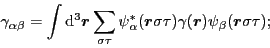
The CE now results from specifying $\eta G$ to the local gauge transformation [13,Dobaczewski and Dudek(1995)] that is defined as

$$\psi'_\alpha({\bm r}\sigma\tau) \equiv (U\psi_\alpha)({\bm r... ...gma\tau) =e^{i\gamma({\bm r})}\psi_\alpha({\bm r}\sigma\tau) .$$ (21)

Then, Eq. (13) gives:

$$\rho'({\bm r}\sigma\tau,{\bm r}'\sigma'\tau',t) = e^{i\left(... ... r}')\right)} \rho({\bm r}\sigma\tau,{\bm r}'\sigma'\tau',t) .$$ (22)

Matrix elements of the local-gauge angle $\gamma({\bm r})$ are given by local integrals,

$$\gamma_{\alpha\beta} = \int {\rm d}^3\bm{r}\sum_{\sigma\tau}... ...m r}\sigma\tau) \gamma({\bm r})\psi_\beta({\bm r}\sigma\tau) ;$$ (23)

therefore, from Eq. (13) again, the average value of the gauge angle, $\langle\gamma\rangle=\mbox{Tr}\gamma\rho$, depends on the scalar-isoscalar local density $\rho_0^0({\bm r},t)=\sum_{\sigma\tau}\rho({\bm r}\sigma\tau,{\bm r}\sigma\tau,t)$, that is,

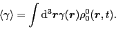$$\langle\gamma\rangle = \int {\rm d}^3\bm{r} \gamma({\bm r})\rho_0^0({\bm r},t) .$$ (24)

Now, the assumed local-gauge invariance of the potential energy implies the equation of motion for the average value $\langle\gamma\rangle$, which from Eq. (20) reads

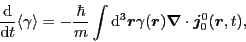$$\frac{{\rm d}}{{\rm d} t}\langle\gamma\rangle = -\frac{\hba... ...^3\bm{r}\gamma({\bm r}) \bm{\nabla}\cdot\bm{j}_0^0(\bm{r},t) ,$$ (25)

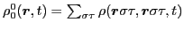
where the standard scalar-isoscalar current is defined as [16] $\bm{j}_0^0({\bm r},t)=\sum_{\sigma\tau}\frac{1}{2i} \left[({\bm\nabla}-{\bm\nabla}') \rho({\bm r}\sigma\tau,{\bm r}'\sigma\tau,t)\right]_{{\bm r}={\bm r}'}$.

We note here [13,Dobaczewski and Dudek(1995)], that the gauge invariance that corresponds to a specific dependence of the gauge angle on position, $\gamma({\bm r})={\bm P}_0\cdot{\bm r}$, represents the Galilean invariance of the potential energy for the system boosted to momentum ${\bm P}_0$. Then, equation of motion (25) simply represents the classical equation for the center-of-mass velocity,

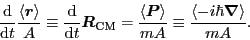$$\frac{{\rm d}}{{\rm d} t}\frac{\langle{\bm r}\rangle}{A} \e... ...le}{mA} \equiv \frac{\langle -i\hbar{\bm\nabla}\rangle}{mA} .$$ (26)

In the general case, that is, when the potential energy is gauge-invariant and the gauge angle $\gamma({\bm r})$ is an arbitrary function of ${\bm r}$, Eq. (25) gives the CE that reads

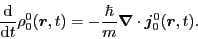$$\frac{{\rm d}}{{\rm d} t} \rho_0^0({\bm r},t) = -\frac{\hbar}{m} \bm{\nabla}\cdot\bm{j}_0^0(\bm{r},t) .$$ (27)

Thus for a gauge-invariant potential energy density, the TDHF or TDDFT equation of motion implies the CE, that is, the gauge invariance is a sufficient condition for the validity of the CE. By proceeding in the opposite direction, we can prove that it is also a necessary condition. Indeed, the CE of Eq. (27) implies the first-order condition (19), and then the full gauge invariance stems from the fact that the gauge transformations form local U(1) groups.