The N$^{3}$LO quasilocal functional

We are now in a position to discuss the CE for the N$^{3}$LO quasilocal functional introduced by Carlsson et al. [Carlsson et al.(2008)Carlsson, Dobaczewski, and Kortelainen]. By imposing on the functional the gauge-invariance conditions, we can then confirm and explicitly rederive the results of Sec. 2.2. The explicit derivation will also allow us to discuss the CEs for densities in other spin-isospin channels analyzed in Sec. 2.2.2.

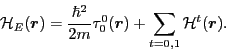
Below we consider the EDF given in terms of a local integral of the energy density $\mathcal{H}_E(\bm{r})$,

$$E\{\rho\} = \int {\rm d}^3\bm{r} \ \mathcal{H}_E(\bm{r}) ,$$ (32)

which is represented as a sum of the kinetic and potential energies conforming to Eq. (11),

$$\mathcal{H}_E(\bm{r})= \frac{\hbar^{2}}{2 m} \tau_0^0(\bm{r}) + \sum_{t=0,1} \mathcal{H}^t(\bm{r}) .$$ (33)

To lighten the notation and avoid confusion with the isospin index $t=0,1$, in this section we do not explicitly show the time argument of densities, which within the TDDFT all depend on time.

The quasilocal N$^{3}$LO EDF was constructed [Carlsson et al.(2008)Carlsson, Dobaczewski, and Kortelainen] by building the $t=0$ and $t=1$ potential-energy densities $\mathcal{H}^t(\bm{r})$ from isoscalar and isovector densities, respectively, and their derivatives up to sixth order. For clarity, we give here a brief summary of definitions and notations used in this construction.

The local higher-order primary densities are defined by the coupling of relative-momentum tensors $K_{n L}$ [Carlsson et al.(2008)Carlsson, Dobaczewski, and Kortelainen] with nonlocal densities (29) to total angular momentum ${J}$, that is,

$$\rho_{n L v J}^t(\bm{r})= \left\{ \left[ K_{n L} \rho_{v}^t(\bm{r}, \bm{r}') \right]_{J} \right\}_{\bm{r}'= \bm{r}} .$$ (34)

Then, a general term of the N$^{3}$LO functional can be written, in the language of the spherical tensors, as

$$T_{m I, n L v J}^{n' L' v' J',t} (\bm{r}) \!\!=\!\! \left[\left[ ... ...ft[D_{m I} \rho_ {n L v J}^t(\bm{r}) \right]_{J'} \right]^{0} \right]_{0}\!\! ,$$ (35)

where the local secondary densities, $\left[D_{m I} \rho_ {n L v J}^t(\bm{r})\right]_{J'}$, are obtained by acting with derivatives $D_{m I}$ on primary densities and coupling them to total angular momentum ${J'}$. Each term (35) is multiplied by the corresponding coupling constant $C_{m I, n L v J}^{n' L' v' J',t}$ that is denoted by the same set of indices as those in the term itself.

We note here that the definition of the isovector terms depends on whether one uses Cartesian or spherical representation of tensors in isospace. On the one hand, the use of the standard Cartesian representation, see, e.g., Refs. [16,Carlsson et al.(2008)Carlsson, Dobaczewski, and Kortelainen], implies that the isovector terms depend on products of differences of neutron and proton densities. On the other hand, the use of the spherical representation, which was assumed in Ref. [Raimondi et al.(2011)Raimondi, Carlsson, and Dobaczewski] and is also used in the present study, involves the coupling of two isovectors to a scalar, whereby there appears a Clebsch-Gordan coefficient of $\left(\sqrt{3}\right)^{-1}$. Therefore, for the isospace spherical representation, the isovector coupling constants are by the factor of $\left(\sqrt{3}\right)$ larger than those for the Cartesian representation.

In the remaining part of this section, we employ the compact notation introduced in Ref. [11], whereby the grouped indices, such as the Greek indices $\alpha=\left\{ n_{\alpha}L_{\alpha}v_{\alpha}J_{\alpha}\right\}$ and the Roman indices $a=\left\{m_aI_a\right\}$, denote all the quantum numbers of the local densities $\rho_{\alpha}(\bm{r})$ and derivative operators $D_{a}$, respectively. In this notation, the N$^{3}$LO potential-energy density of Eq. (33) reads

$${\cal H}^t(\bm{r})=\sum_{a\alpha\beta}C_{a,\alpha}^{\beta,t}T_{a,\alpha}^{\beta,t}(\bm{r}).$$ (36)

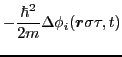
Our following discussion of the CE is mainly focused on the one-body potential-energy term, defined in Eq. (16) as the variation of the potential energy with respect to the density matrix. For the N$^{3}$LO functional, this term was derived in Ref. [11], where it was shown that in space coordinates it has the form of a one-body pseudopotential,

$$\hat{\Gamma}^{\sigma\sigma'}_{\tau\tau'}(\bm{r})= \sum_{\gam... ...ight]_{J_{\gamma}}\right]_{0}\tau^{t}_{\tau\tau'}\right]^{0} .$$ (37)

An equivalent form of the one-body pseudopotential, which can be obtained by recoupling spherical tensors within a scalar, and which separates out the spin Pauli matrices, reads

$$\hat{\Gamma}^{\sigma\sigma'}_{\tau\tau'}(\bm{r})= \sum_{\gam... ...ma'}_{v_{\gamma}}\right]_{0} \tau^{t}_{\tau\tau'}\right]^{0} .$$ (38)

In turn, potentials $U_{\gamma}^{t}(\bm{r})$ were derived as linear combinations of the secondary densities,

$$U_{\gamma}^{t}(\bm{r})=\sum_{a\alpha\beta;d\delta} C_{a,\alp... ...ta} \left[D_{d}\rho^{t}_{\delta}(\bm{r})\right]_{J_{\gamma}} ,$$ (39)

where $\chi_{a,\alpha;\gamma}^{\beta;d\delta}$ are numerical coefficients. We call the one-body operator $\hat{\Gamma}^{\sigma\sigma'}_{\tau\tau'}(\bm{r})$ pseudopotential, because it is defined in terms of potentials $U_{\gamma}^{t}(\bm{r})$ and differential operators $D_{n_{\gamma}L_{\gamma}}$ acting on single-particle wave functions. We note here, that in Eqs. (37) and (38) potentials always appear to the left of all derivatives; nonetheless, the one-body pseudopotential is a hermitian operator, which is guaranteed by specific conditions obeyed by potentials $U_{\gamma}^{t}(\bm{r})$, which were derived in Ref. [11].

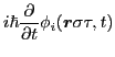
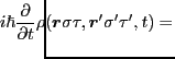
For the one-body pseudopotential (37), the Schrödinger equation that gives the time evolution of single-particle Kohn-Sham wave functions in space coordinates reads,

$$i\hbar\frac{\partial}{\partial t}\phi_{i}(\bm{r}\sigma\tau,t) = -\frac{\hbar^{2}}{2m}\Delta\phi_{i}(\bm{r}\sigma\tau,t)$$

$$+ \sum_{\sigma'\tau'}\hat{\Gamma}^{\sigma\sigma'}_{\tau\tau'}(\bm{r}) \phi_{i}(\bm{r}\sigma'\tau',t) .$$ (40)

By multiplying the Schrödinger equation with the complex-conjugated wave function, $\phi^*_{i}(\bm{r}'\sigma'\tau',t)$ and summing over the single-particle index $i$ we obtain the time-evolution equation of the density matrix (14), that is,

$$\hspace{-1cm}i \hbar \frac{\partial}{\partial t}\rho(\bm{r} \sigma \tau, \bm{r}' \sigma' \tau' ,t) =$$

$$-\frac{\hbar^2}{2m}\left(\Delta-\Delta'\right) \rho(\bm{r} \sigma \tau, \bm{r}' \sigma' \tau' ,t)$$

$$+ \sum_{\sigma''\tau''}\left( \hat{\Gamma}^{\sigma\sigma''}_{\tau\tau''}(\bm{r}) \rho(\bm{r} \sigma''\tau'', \bm{r}' \sigma' \tau' ,t) \right.$$

$$\hspace{0.9cm} - \left. \hat{\Gamma}^{\sigma'\sigma''*}_{\tau'\tau''}(\bm{r}') \rho(\bm{r} \sigma \tau, \bm{r}' \sigma'' \tau'' ,t)\right) .$$ (41)

Before we proceed, we must first consider the complex-conjugated pseudopotential $\hat{\Gamma}^{\sigma'\sigma''*}_{\tau'\tau''}(\bm{r}')$. To this end, we use the property of the Biedenharn-Rose phase convention employed in Refs. [Carlsson et al.(2008)Carlsson, Dobaczewski, and Kortelainen,11], by which all scalars are always real. Note that for the spherical representation of Pauli matrices, the Biedenharn-Rose phase convention implies the transposition of spin indices, that is,

$$\left(\sigma^{\sigma\sigma'}_{v\mu}\right)^* = (-1)^{v-\mu} \sigma^{\sigma'\sigma}_{v,-\mu} ,$$ (42)

where $\mu=0$ for $v=0$ and $\mu=-1,0,1$ for $v=1$ denote tensor components of scalar and vector Pauli matrices, respectively.

Finally, in Eqs. (38) and (39), the complex conjugation only affects coefficients $\chi_{a,\alpha;\gamma}^{*\beta;d\delta}= (-1)^{n_\gamma+m_a+m_d}\chi_{a,\alpha;\gamma}^{\beta;d\delta}$ [11], which gives,

$$\hat{\Gamma}^{\sigma'\sigma''*}_{\tau'\tau''}(\bm{r}') = \hat{\Gamma}^{'\sigma''\sigma'}_{\tau''\tau'}(\bm{r}') ,$$ (43)

for

$$\hat{\Gamma}^{'\sigma\sigma'}_{\tau\tau'}(\bm{r}')= \sum_{\g... ...igma'}_{v_{\gamma}}\right]_{0} \tau^{t}_{\tau\tau'}\right]^{0}$$ (44)

and

$$U_{\gamma}^{'t}(\bm{r}')=\sum_{a\alpha\beta;d\delta} (-1)^{n... ...} \left[D'_{d}\rho^{t}_{\delta}(\bm{r}')\right]_{J_{\gamma}} .$$ (45)

It means that in all further derivations we must use the second set of potentials $U_{\gamma}^{'t}(\bm{r}')$ with signs of terms modified according to the phase $(-1)^{n_\gamma+m_a+m_d}$. It is now obvious that the CEs will hold independently of the spin-isospin coordinates if, and only if, the pseudopotentials fulfill the condition

$$\sum_{\sigma''\tau''}\left(\Gamma_{\tau\tau''}^{\sigma\sigma''}(\mathbf{r})\rho(\mathbf{r}\sigma''\tau'',\mathbf{r'}\sigma'\tau') \right.$$

$$~~~~~~ \left. -\Gamma_{\tau''\tau'}^{'\sigma''\sigma'}(\mathbf{r}')\rho(\mathbf{r}\sigma\tau,\mathbf{r'}\sigma''\tau'')\right)_{\bm{r}'=\bm{r}}=0 .$$ (46)

We are now in a position to separate the four spin-isospin channels in Eq. (41). We do so by multiplying both sides of the equation with $\sigma_v^{\sigma'\sigma}\tau_{\tau'\tau}^t$ and summing over $\sigma \tau,\sigma' \tau'$. From Eq. (29) it is then obvious that, in close analogy to Sec. 2.1, after setting $\bm{r}'=\bm{r}$, we obtain the CEs (30) in the four spin-isospin channels, provided terms coming from one-body pseudopotentials do not contribute, as in Eq. (46). When evaluating this condition for the four spin-isospin channels, we use the expression for the trace of three Paul matrices in spherical representation, which reads [17],

$${\rm Tr}\Big[\sigma_{v\mu}\sigma_{v'\mu'}\sigma_{v''\mu''}\Big] =A(v+v'+v'')(-1)^{v-\mu}C^{v,-\mu}_{v'\mu'v''\mu''} ,$$ (47)

where we introduced $A(v+v'+v'')$ as a shorthand symbol for numerical coefficients coming from the computation of the trace. In the calculation, we only need values of $A(0)=2$, $A(2)=2\sqrt{3}$, $A(3)=2\sqrt{2}\,i$. After a trivial but lengthy calculation, we obtain the final result:

$$\hspace*{-1cm}\sum_{v't', \gamma,t''J} A(v+v'+v_{\gamma})A(t+t'+t... ...{ccc} J_{\gamma} & L_{\gamma} & v_{\gamma} \\ v' & v & J \end{array}\right\}$$

$$\hspace*{-1cm}\times\bigg( \left[\left[U_{\gamma}^{t''}(\mathbf{r... ...{v'}^{t'}(\bm{r},\bm{r}')\right]_J\right]_v\right]^t \bigg)_{\bm{r}'=\bm{r}}=0.$$ (48)

For our practical implementation of the CE condition (48), we proceed by transforming the two differential operators, $D_{n_{\gamma}L_{\gamma}}$ and $D'_{n_{\gamma}L_{\gamma}}$, which act on two different variables $\bm{r}$ and $\bm{r}'$, respectively, with the recoupling methods developed in Ref. [11], and we obtain,

$$D_{n_{\gamma}L_{\gamma}} = \sum_{nLn'L'}K_{nLn'L'}^{n_{\gamma}L_{\gamma}} (i)^{n}2^{-n'}\left[D_{n'L'}K_{nL}\right]_{L_{\gamma}},$$ (49)

$$D'_{n_{\gamma}L_{\gamma}} = \sum_{nLn'L'}K_{nLn'L'}^{n_{\gamma}L_{\gamma}} (-i)^{n}2^{-n'}\left[D_{n'L'}K_{nL}\right]_{L_{\gamma}}.$$ (50)

On the right-hand sides, operators $K_{n L}$ are the higher-order spherical tensor derivatives [Raimondi et al.(2011)Raimondi, Carlsson, and Dobaczewski] built of the relative momenta, $\bm{k}=(\bm{\nabla}-\bm{\nabla}')/2i$, and operators $D_{n'L'}$ act on variable $\bm{r}$ after one sets $\bm{r}'=\bm{r}$. The 91 numerical coefficients $K_{nLn'L'}^{n_{\gamma}L_{\gamma}}$, which are needed up to N$^{3}$LO, have been derived in Ref. [11]. By using Eqs. (49) and (50), one can express the last line of the Eq. (48) as a linear combination of products of pairs of secondary densities coupled in the spin and isospin spaces to ranks $v$ and $t$, respectively. This final form, which for brevity is not shown here explicitly, is used in obtaining the results of Sec. 3.