Determination of parameters

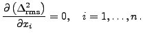
The function (2) has an extremum when all its partial derivatives with respect to the model parameters $x_i$ are simultaneously zero,

$$\frac{\partial\left(\Delta_{\text{rms}}^2\right)}{\partial x_i} = 0, \quad i=1,\ldots,n \,.$$ (3)

These partial derivatives are in general non-linear functions of the model parameters; thus to get manageable equations, Eq. (1) has to be linearized, i.e.,

$$f_j({\vec x}) \simeq f_j({\vec x}_0) + \sum_{i=1}^n \left(\frac{\partial f_j}{\partial x_i}\right)_{{\vec x}={\vec x}_0} (x_i - x_{0,i})\,.$$ (4)

For observables related to total or single-particle energies, the non-linearities can actually be quite small [4,10], but in general this is not the case and the linearized equations have to be solved iteratively.

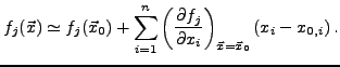
We now introduce the notation that ${\vec x}_0$ is the set of parameters from previous iteration, by which $x_i-x_i^0$ is the change of parameters to be determined. We also denote the weighted deviations of observables from experiment by $y_j$,

$$y_j \equiv \sqrt{W_j}\left(e_j^{\text{exp}} - f_j({\vec x}_0)\right)\,,$$ (5)

and the weighted matrix of regression coefficients is denoted as

$$J_{ji} \equiv \sqrt{W_j}I_{ji}$$ (6)

for

$$I_{ji} = \left(\frac{\partial f_j}{\partial x_i}\right)_{{\vec x}={\vec x}_0}.$$ (7)

Then, Eq. (2) can be written as

$$\Delta^2_{\text{rms}} = \frac{1}{m-n} \sum_{j=1}^m \left( \sum_{i=1}^n J_{ji} (x_i-x_i^0) - y_j \right)^2\,,$$ (8)

and Eq. (3) takes the form:

$$\left(J^T J\right) ({\vec x}-{\vec x}_0) = J^T {\vec y}\,.$$ (9)

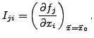
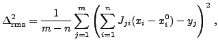
It is now obvious that the parameters lying in the null space of $J^T J$ (if it is singular) cannot be determined. Moreover, during the fitting procedure it often happens that some parameters are very poorly determined by the experimental data. These parameters should be removed from the set because they have very large uncertainties and, if kept, would destroy the subsequent error analysis (see below). The poorly determined parameters can be found by first transforming to a new set of parameters, here called 'independent parameters' and then eliminating all non-important independent parameters from the fit.

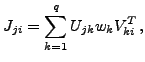
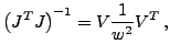
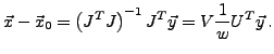
This can be achieved by making a singular value decomposition (SVD) [17] of matrix $J$,

$$J_{ji} = \sum_{k=1}^q U_{jk} w_k V^T_{ki}\,,$$ (10)

where columns of the $m \times q$ matrix $U$ are orthogonal ($U^TU=1$), columns of the $n \times q$ matrix $V$ are also orthogonal ($V^TV=1$), and $q$ positive numbers $w_k$ are called singular values of $J$. Note that for singular matrix $J^T J$ one has $q<n$, and the vanishing singular values do not contribute to the sum in Eq. (10).

The SVD of $J$ allows one to calculate the inverse $\left(J^TJ\right)^{-1}$ outside the null space of $J^TJ=Vw^2V^T$,

$$\left(J^TJ\right)^{-1}=V\frac{1}{w^2}V^T\,,$$ (11)

and the solution of Eq. (9) can now be expressed as

$${\vec x}-{\vec x}_0 = \left(J^TJ\right)^{-1}J^T {\vec y} = V\frac{1}{w}U^T {\vec y}\,.$$ (12)

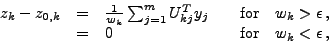
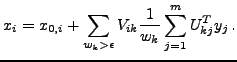
The new independent parameters are now defined as ${\vec z} = V^T {\vec x}$. If some singular values become very small, the associated variables are simply dropped from Eq. (12), i.e.,

$$\begin{array}{rclll} z_k-z_{0,k} &=& \frac{1}{w_k}\sum_{j=1}^... ...ilon\,,\\ &=& 0 &\quad\mbox{for}& w_k < \epsilon\,, \end{array}$$ (13)

and the new parameters $x_i$ become

$$x_i = x_{0,i}+\sum_{w_k > \epsilon} V_{ik} \frac{1}{w_k}\sum_{j=1}^m U^T_{kj} y_j\,.$$ (14)

These new values can now be used to continue iterations.