After the iteration has converged, one can determine error estimates
for the obtained parameters ![]() . The method used here follows the
standard multivariate regression analysis [18,19]
Assume that we take the scaled experimental observables and perturb
them with a random noise that has zero mean value. The true
experimental energies can now be thought of as being random variables
but only one sample that has the values
. The method used here follows the
standard multivariate regression analysis [18,19]
Assume that we take the scaled experimental observables and perturb
them with a random noise that has zero mean value. The true
experimental energies can now be thought of as being random variables
but only one sample that has the values
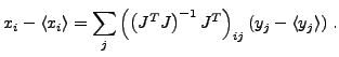
![]() is known. The deviation of each
model parameter
is known. The deviation of each
model parameter ![]() from its mean can then be calculated from
Eq. (12) as
from its mean can then be calculated from
Eq. (12) as
The average values of parameters
![]() are
determined by the least square fitting procedure,
are
determined by the least square fitting procedure,
![]() . It is also assumed that the least square fitting gives
an accurate estimate of the standard deviation of the observables
. It is also assumed that the least square fitting gives
an accurate estimate of the standard deviation of the observables
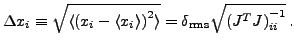
![]() . With these assumptions from Eq. (16) we get the
following formula for the confidence interval of
. With these assumptions from Eq. (16) we get the
following formula for the confidence interval of ![]() with
with
![]() probability:
probability:
We have to stress at this point that the error estimates of
Eq. (19) have quite different meaning for the exact and
inaccurate models discussed at the beginning of this section. In the
first case, errors of the parameters result solely from the statistical
noise in the measured observables--their variances are supposed to be
known and define the weights in Eq. (2) as
![]() . Therefore, within the exact
model, the assumption of equal variances, Eq. (18), is well
justified. Such a model then gives the minimum value of
. Therefore, within the exact
model, the assumption of equal variances, Eq. (18), is well
justified. Such a model then gives the minimum value of
![]() near 1, i.e. the
near 1, i.e. the ![]() test.
test.
For
a inaccurate model, the error estimates of Eq. (19) only
give information on the sensitivity of the model parameters to the values
of the observables. They correspond to the situation where the
experimental values are artificially varied far beyond their
experimental uncertainties, so as to induce tangible variations in the
values of the parameters. Eq. (18) then means that the range of
this variation is inversely proportional to
![]() , i.e. it
is commensurate with the importance attributed to a given observable.
Here, the error estimates may depend on the weights, and are thus
affected by their choices, and similarly so are the values of the parameters.
, i.e. it
is commensurate with the importance attributed to a given observable.
Here, the error estimates may depend on the weights, and are thus
affected by their choices, and similarly so are the values of the parameters.
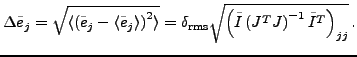
We are now in a position to discuss the mass predictions and error propagation. Suppose that we apply the model of Eq. (1) not only to the measured masses but also to the masses of unknown nuclei,
The error estimates of Eq. (19) allow us to estimate
uncertainties of the predicted observables.
With the same assumptions as before, but now with
the parameters ![]() from the least square fit for both observables inside and
outside the fitted set, we get
from the least square fit for both observables inside and
outside the fitted set, we get
Equations (19) and (22) form the basis of the error
analysis of our mass fits. The calculated error bars (19) of parameters ![]() must then be further scrutinized to analyze which
parameters are necessary and which should be removed from the model.
The confidence intervals (22) constitute estimates of
predictivity of the model. Note that they should also be calculated
for the observables that have actually been used in the fit. It is
these intervals, and not the residuals
must then be further scrutinized to analyze which
parameters are necessary and which should be removed from the model.
The confidence intervals (22) constitute estimates of
predictivity of the model. Note that they should also be calculated
for the observables that have actually been used in the fit. It is
these intervals, and not the residuals
![]() , which have to be
analyzed when discussing the quality of the model. It is
obvious that the residuals can be arbitrarily small for some
observables, or for some types of observables (e.g., masses of
semimagic spherical nuclei), while the model can still be quite
uncertain in describing these same observables.
, which have to be
analyzed when discussing the quality of the model. It is
obvious that the residuals can be arbitrarily small for some
observables, or for some types of observables (e.g., masses of
semimagic spherical nuclei), while the model can still be quite
uncertain in describing these same observables.