


Next: Constraints
Up: Skyrme Hartree-Fock-Bogoliubov Method
Previous: Lipkin-Nogami Method
Particle-Number Projection After Variation
Introducing the particle-number projection operator for  particles,
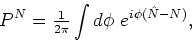 |
(68) |
where  is the number operator, the average HFB energy of the
particle-number projected state can be expressed as an integral over the
gauge angle
is the number operator, the average HFB energy of the
particle-number projected state can be expressed as an integral over the
gauge angle  of the Hamiltonian matrix elements between states
with different gauge angles [37,38]. In particular, for the Skyrme-HFB
method implemented here, the particle-number projected
energy can be written as [26,25]
of the Hamiltonian matrix elements between states
with different gauge angles [37,38]. In particular, for the Skyrme-HFB
method implemented here, the particle-number projected
energy can be written as [26,25]
![\begin{displaymath}
\textsf{E}^{N}[\rho,\tilde{\rho}]=\frac{\left\langle \Phi \v...
...\int d\phi ~y(\phi )\int d^3{\bf r}~{\cal H}({\bf r},\phi )~,
\end{displaymath}](img211.png) |
(69) |
where the gauge-angle dependent energy density
 is derived from the unprojected energy density
 (10) by simply substituting the
particle and pairing local densities
(10) by simply substituting the
particle and pairing local densities
 ,
,
 ,
,
 , and
, and
 by their gauge-angle
dependent counterparts
by their gauge-angle
dependent counterparts
 ,
,
 ,
,
 , and
, and
 , respectively.
The latter densities are calculated from the gauge-angle dependent density matrices as
, respectively.
The latter densities are calculated from the gauge-angle dependent density matrices as
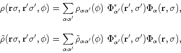 |
(70) |
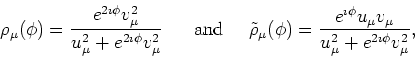
where the gauge-angle dependent matrix elements read
 |
(71) |
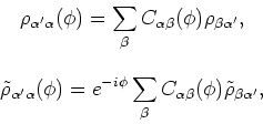
and depend on the unprojected matrix elements (47) and
on the gauge-angle dependent matrix
![\begin{displaymath}
C(\phi ) =e^{2i\phi }\left[ 1+\rho (e^{2i\phi }-1)\right]^{-1}.
\end{displaymath}](img220.png) |
(72) |
Function  appearing in Eq. (69) is defined as
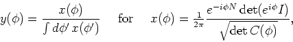 |
(73) |
where  is the unit matrix.
Since the gauge-angle dependent matrices (70) and
(71) are all diagonal in the same canonical basis that
diagonalizes the unprojected density matrices (47),
all calculations are very much simplified when they are performed in
the canonical basis. In particular, in the canonical basis the
matrices (71) read
 |
(74) |
while the function  can be calculated as
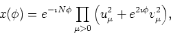 |
(75) |
where  and
and  (
(
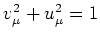 ) are the usual
canonical basis occupation amplitudes.
) are the usual
canonical basis occupation amplitudes.
All the above expressions apply to independently restoring the proton and neutron numbers,
so, in practice, integrations over two gauge angles have to be
simultaneously implemented. In practice, these integrations are
carried out by using a simple discretization method, which amounts
to approximating the projection operator (68) by a
double sum [39], i.e.,
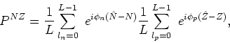 |
(76) |
where
 |
(77) |
Usually no more than  points are required for a precise
particle number restoration.
points are required for a precise
particle number restoration.
Next: Constraints
Up: Skyrme Hartree-Fock-Bogoliubov Method
Previous: Lipkin-Nogami Method
Jacek Dobaczewski
2004-06-25