Calculations of Matrix Elements

As discussed in Sect. 3.2, local densities (25) and average fields, (17) and (18), are calculated in the coordinate space. Therefore, calculation of matrix elements (38) amounts to calculating appropriate spatial integrals in the cylindrical coordinates $r$ and $z$. In practice, the integration is carried out by using the Gauss quadratures [31] for 22 Gauss-Hermite points in the $z>0$ direction and 22 Gauss-Laguerre points in the $r$ direction. This gives a sufficient accuracy for calculations up to $N_{sh}=40$.

In the case of the HO basis functions, the integration is performed by using the Gauss integration points, $\xi_n$ and $\eta_m$, for which the local densities and fields have to be calculated at the mesh points of $z_n$=$b_z\xi_n$ and $r_m$= $b_\bot\eta_m^{1/2}$. As an example, consider the following diagonal matrix element of the potential $U_q(r,z)$ (18),

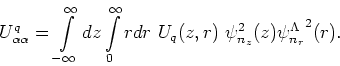$$U^q_{\alpha\alpha}=\int\limits_{-\infty}^{\infty} dz\int\lim... ...} r d r~ U_q(z,r)~\psi_{n_{z}}^2(z) {\psi_{n_r}^\Lambda}^2(r).$$ (39)

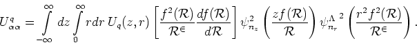
Inserting here the HO functions $\psi_{n_{z}}^2(z)$ and ${\psi_{n_r}^\Lambda}^2(r)$ (29), and changing the integration variables to dimensionless variables $\xi$ and $\eta$, the above matrix element reads

$$U^q_{\alpha\alpha}=\int\limits_{-\infty} ^{\infty}d\xi\int\l... ...ilde{\psi}_{n_z}^2 (\xi) \tilde{\psi}_{n_r}^{\Lambda~2}(\eta),$$ (40)

where

$$\tilde{U}_q(\xi,\eta)={\textstyle{\frac{1}{2}}} U_q(\xi b_z,\sqrt{\eta}\, b_\bot).$$ (41)

Here, the Gauss integration quadratures can be directly applied, because the HO wave functions contain appropriate exponential profile functions.

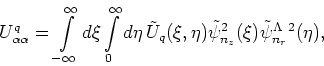
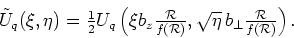
The situation is a little bit more complicated in the case of the THO basis states where, before calculating, one has to change variables with respect to the LST functions $f({\cal R})$. For example, let us consider the same matrix elements (39) but in THO representation:

$$U^q_{\alpha\alpha}= \displaystyle \int\limits_{-\infty}^{\in... ...left( \frac{r^{2}f^{2}(\mathcal{R})}{\mathcal{R}^{2}}\right) .$$ (42)

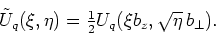
Introducing new dimensionless variables

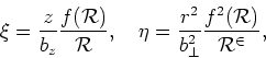$$\displaystyle \xi=\frac{z}{b_{z}}\frac{f(\mathcal{R})}{\math... ...^{2}}{b_{\bot}^{2}}\frac{f^{2}(\mathcal{R})}{\mathcal{R}^{2}},$$ (43)

for which we have

$$d\xi~d\eta=\frac{2}{b_{z}b_{\bot}^{2}}\left[ \frac{f^{2}(\ma... ...{R}^{2}}\frac{df(\mathcal{R})}{d\mathcal{R}}\right] r d r~ dz,$$ (44)

the matrix elements have the form of integrals, which are exactly identical to those in the HO basis (40), after changing the function $\tilde{U}_q(\xi,\eta)$ to

$$\tilde{U}_q(\xi,\eta)={\textstyle{\frac{1}{2}}} U_q\left(\x... ...b_\bot{\textstyle{\frac{\mathcal{R}}{f(\mathcal{R})}}}\right).$$ (45)

The calculation of matrix elements corresponding to derivative terms in the Hamiltonian (17) can be performed in an analogous way, after the derivatives of the Jacobian, ${\textstyle{\frac{f^{2}(\mathcal{R} )}{\mathcal{R}^{2}}}}{\textstyle{\frac{df(\mathcal{R})}{d\mathcal{R}}}}$, are taken into account.