Isospin projection formalism

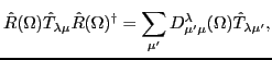
Within the MF approximation, the isospin symmetry breaking has two sources. The spontaneous breaking of isospin associated with the MF approximation itself [36,26,29] is, in this theory, intertwined with the explicit symmetry breaking due to the Coulomb interaction. The essence of our method [28,29] is to retain the explicit isospin mixing. 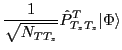It is achieved by rediagonalizing the total effective nuclear Hamiltonian $\hat H_{NN}$ in good-isospin basis. 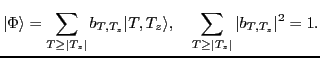The basis is generated by using the projection-after-variation technique, that is, by acting with the standard one-dimensional isospin-projection operator on the MF product state $\vert\Phi\rangle$:

$$\vert TT_z\rangle = \frac{1}{\sqrt{N_{TT_z}}}\hat{P}^T_{T_z T_z} \vert\Phi\rangle$$

$$= \frac{2T+1}{2 \sqrt{N_{TT_z}}}\int_0^\pi d\beta\sin\beta \; d^{T}_{T_z T_z}(\beta)\; \hat{R}(\beta)\vert\Phi\rangle,$$ (1)

where $\beta$ denotes the Euler angle associated with the rotation operator $\hat{R}(\beta)= e^{-i\beta \hat{T}_y}$ about the $y$-axis in the isospace, $d^{T}_{T_z T_z}(\beta)$ is the Wigner function [37], and $T_z =(N-Z)/2$ is the third component of the total isospin $T$. The wave function $\vert\Phi\rangle$ is obtained self-consistently by solving the Skyrme-Hartree-Fock (SHF) equations. In the HF limit, the $z$-component $T_z$ is strictly conserved. The overlap $N_{T T_z}$, or interchangeably the normalization factor $b_{T,T_z}$, are given by

$$N_{T T_z} \equiv b_{T,T_z}^2 = \langle \Phi \vert \hat{P}^T_{T_z T_z} \vert \Phi \rangle$$

$$= \frac{2T+1}{2}\int_0^\pi d\beta \sin\beta \; d^{T}_{T_z T_z} (\beta ) \; {\mathcal N}(\beta),$$ (2)

where

$${\mathcal N}(\beta) = \langle \Phi\vert \hat{R}(\beta)\vert \Phi\rangle$$ (3)

stands for the overlap kernel. The good-isospin basis is spanned by the states $\vert T,T_z\rangle$ that have tangible contributions to the MF state

$$\vert\Phi \rangle = \sum_{T\geq \vert T_z\vert} b_{T,T_z} \vert T,T_z\rangle , \quad \sum_{T\geq \vert T_z\vert} \vert b_{T,T_z}\vert^2 = 1.$$ (4)

In practice, we retain states having $\vert b_{T,T_z}\vert^2>10^{-10}$, which sets the limit of $T\leq \vert T_z\vert+5$.

The total nuclear Hamiltonian consists of the kinetic energy $\hat T$, the Skyrme interaction $\hat V^{S}$ and the Coulomb interaction $\hat V^{C}$ that breaks isospin:

$$\hat H_{NN} = \hat T + \hat V^{S} + \hat V^{C}$$

$$\equiv \hat T + \hat V^{S} +\hat V_{00}^C + \hat V_{10}^C + \hat V_{20}^C ,$$ (5)

where

$$\hat V_{00}^C(r_{ij}) = \; \; \; \frac{1}{4}\frac{e^2}{r_{ij}} \left( 1 + \frac{1}{3} \hat {\tau}^{(i)} \circ \hat {\tau}^{(j)} \right)$$ (6)

$$\hat V_{10}^C(r_{ij}) = - \frac{1}{4}\frac{e^2}{r_{ij}} \left( \hat \tau_{10}^{(i)} + \hat \tau_{10}^{(j)} \right)$$ (7)

$$\hat V_{20}^C(r_{ij}) = \; \; \; \frac{1}{4}\frac{e^2}{r_{ij}} \; \left( \hat \tau_{10}^... ...{10}^{(j)} - \frac{1}{3} \hat {{\tau}}^{(i)} \circ \hat {{\tau}}^{(j)} \right)$$ (8)

are, respectively, isoscalar, covariant rank-1 (isovector), and covariant rank-2 axial (isotensor) spherical tensor components of the Coulomb interaction. They are constructed by coupling spherical components of the one-body isospin operator:

$$\hat \tau_{10} = \hat \tau_{z}, \quad \hat \tau_{1\pm 1} = \mp \frac{1}{\sqrt{2}} \left( \hat \tau_{x} \pm i \hat \tau_{y} \right) ,$$ (9)

where $\hat \tau_{i},\,i=x,y,z$ denote Pauli matrices and symbol $\circ$ stands for the scalar product of isovectors.

The Coulomb interaction is the only source of the isospin symmetry violation in our model. Charge symmetry breaking components of the strong interaction and the isovector kinetic energy (which is quenched as compared to its isoscalar counterpart by a factor $\frac{\Delta M}{M} \sim 0.001$ due to very small mass difference $\Delta M$ between the neutron and the proton relative to mean nucleonic mass $M$) are not taken into account. 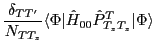Hence, the isoscalar part of the total Hamiltonian reads $\hat H_{00} = \hat T + \hat V^{S} +\hat V_{00}^C$. Its matrix elements can be cast into one-dimensional integrals:

$$\langle T T_z \vert \hat H_{00} \vert T' T_z\rangle = \frac{\delta_{TT'}}{N_{TT_z}} \langle \Phi \vert \hat H_{00} \hat{P}^T_{T_z T_z} \vert \Phi \rangle$$

$$= \frac{\delta_{TT'}}{N_{TT_z}} \frac{2T+1}{2}\int_0^\pi d\beta \sin\beta \; d^{T}_{T_z T_z}(\beta ) \; {\mathcal H}_{00}(\beta) ,$$ (10)

involving the Hamiltonian kernel

$${\mathcal H_{00}}(\beta) = \langle \Phi\vert\hat{H}_{00} \hat{R}(\beta)\vert \Phi\rangle.$$ (11)

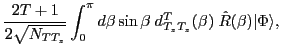
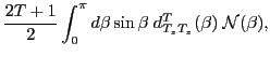
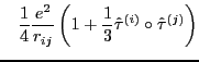
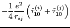
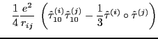
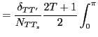
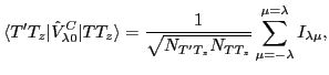
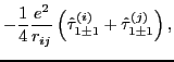
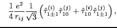
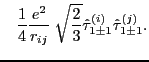
Calculation of matrix elements of the isovector (7) and isotensor (8) components of the Coulomb interaction is slightly more complicated. It appears, however, that these matrix elements can also be reduced to one-dimensional integrals over the Euler angle $\beta$:

$$\langle T' T_z \vert \hat V^C_{\lambda 0} \vert T T_z \rangle = \... ...{N_{T' T_z} N_{T T_z}}} \sum_{\mu = -\lambda}^{\mu = \lambda} I_{\lambda \mu} ,$$ (12)

where

$$I_{\lambda \mu} = (-1)^\mu C^{T' T_z}_{T T_z \lambda 0} C^{T' T_z}_{T T_z -\mu \lambda \mu}$$ (13)

$$\times \frac{2T +1}{2}\int_0^\pi d\beta \sin\beta \; d^{T}_{T_z-\mu T_z}(\beta)\; \langle\Phi \vert \hat V^C_{\lambda \mu } \hat{R}(\beta)\vert\Phi\rangle ,$$

and symbols $C^{T K}_{T M \lambda \mu}$ stand for the Clebsch-Gordan coefficients [37]. The non-axial ($\mu$$\ne$0) isovector and isotensor components of the Coulomb interaction appearing in Eq. (13) are:

$$\hat V^C_{1\pm 1}(r_{ij}) = - \frac{1}{4}\frac{e^2}{r_{ij}} \left( \hat \tau_{1\pm 1}^{(i)} + \hat \tau_{1\pm 1}^{(j)} \right),$$ (14)

$$\hat V^C_{2\pm 1}(r_{ij}) = \; \; \; \frac{1}{4}\frac{e^2}{r_{ij}} \frac{1}{\sqrt3} \left( \... ...t \tau_{1 0}^{(j)} + \hat \tau_{1 0}^{(i)} \hat \tau_{1 \pm 1}^{(j)} \right) ,$$ (15)

$$\hat V^C_{2\pm 2}(r_{ij}) = \; \; \; \frac{1}{4} \frac{e^2}{r_{ij}} \; \sqrt{\frac{2}{3}} \hat \tau_{1\pm 1}^{(i)} \hat \tau_{1\pm 1}^{(j)}.$$ (16)

Equations (12)-(13) can be derived by using the standard transformation rules for a covariant spherical-tensor operator $\hat T_{\lambda \mu}$ of rank-$\lambda$ under the three-dimensional rotation by the Euler angles $\Omega = (\alpha, \beta, \gamma)$, that is,

$$\hat R(\Omega) \hat T_{\lambda \mu} \hat R(\Omega)^\dagger = \sum_{\mu'} D^\lambda_{\mu' \mu} (\Omega) \hat T_{\lambda \mu'},$$ (17)

where the SO(3) projection operator $\hat P^{T}_{K M}(\Omega )$ commutes with spherical tensors as [38]

$$\hat P^{T_f}_{K_f M_f} \hat T_{\lambda \mu} \hat P^{T_i}_{M_i K_i} = \strut$$

$$= C^{T_f M_f}_{T_i M_i \lambda \mu} \sum_{M \mu'} (-1)^{(\mu'-\mu)} C^{T_f K_f}_{T_i M \lambda \mu'} \hat T_{\lambda \mu'} \hat P^{T_i}_{M K_i}.$$ (18)

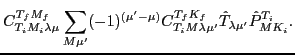
The cornerstone of the isospin projection scheme described above is a calculation of the Hamiltonian and norm kernels and subsequent one-dimensional integration over the Euler angle $\beta$. The integrals are calculated numerically using the Gauss-Legandre quadrature, which is very well suited for this problem provided that the calculated kernels are non-singular.