Isospin structure of the density matrix

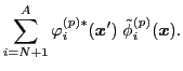
To calculate the transition density matrix and determine its isotopic structure it is convenient to introduce auxiliary ket-states defined as:

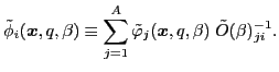$$\tilde{\phi}_i({\boldsymbol x}, q, \beta) \equiv \sum_{j=1}^A\tilde{\varphi}_j({\boldsymbol x}, q, \beta)\; {\tilde O}(\beta)^{-1}_{ji}.$$ (34)

where the space-spin coordinates are abbreviated as ${\boldsymbol x} = ({\boldsymbol r},\sigma )$. This allows for rewriting the transition density matrix into a diagonal form:

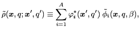$$\tilde{\rho}({\boldsymbol x}, q; {\boldsymbol x}', q') \equiv \su... ...\varphi^*_i({\boldsymbol x}', q')\; \tilde{\phi}_i({\boldsymbol x}, q, \beta ),$$ (35)

where the summation runs over a set of s.p. states, in full analogy with the HF particle density matrix. To alleviate the notation, in what follows we do not indicate the dependence of the transition density matrices on the isorotation angle $\beta$.

An arbitrary matrix in the isospace can be decomposed in terms of the isospin Pauli matrices. In particular, the transition density matrix $\tilde \rho ({\boldsymbol x}, q; {\boldsymbol x}', q')$ can be expressed as:

$$\tilde \rho ({\boldsymbol x}, q; {\boldsymbol x}', q') = \frac{1}{2} \tilde \rho_{00} ({\boldsymbol x}, {\boldsymbol x}') \delta_{q q'}$$

$$+ \frac{1}{2} \sum_{\alpha = 0,\pm 1} \tau_{1\alpha} (q, q') \tilde \rho_{1 \alpha} ({\boldsymbol x}, {\boldsymbol x}'),$$ (36)

where

$$\tau_{10} (q,q') = \langle q \vert \hat \tau_{10} \vert q' \rangle = q \delta_{q,q'} ,$$ (37)

$$\tau_{1\pm 1} (q,q') = \langle q \vert \hat \tau_{1\pm 1} \vert q' \rangle = \mp \sqrt2 \delta_{q, \pm 1} \delta_{q' , \mp 1}.$$ (38)

The isoscalar $\tilde \rho_{00}$ and isovector $\tilde \rho_{1\alpha}$ transition density matrices are calculated by contracting $\tilde \rho$:

$$\begin{eqnarray}\tilde \rho_{00} & = & \; \tilde \rho ,\\ \tilde \rho_{10} & = & \; ( \tau_{10} \tilde \rho ) ,\\ \tilde \rho_{1\pm 1} & = & - \; ( \tau_{1\mp 1} \tilde \rho ). \end{eqnarray}$$ (39a)

The use of the two-dimensional spinor notation is convenient for analytical derivations. However, from the numerical-programming perspective it is better to present expressions in a one-dimensional form, because it allows us to exploit the separability of proton and neutron wave functions and densities - a common feature of essentially all the existing HF codes including the HFODD solver used in this work.

To write the isoscalar and isovector densities in the one-dimensional form we introduce two sets of neutron-like ( $i=1,2,\ldots ,N$) wave functions:

$$\tilde{\phi}_i^{(n)} ({\boldsymbol x}) \equiv \sum_{j=1}^N \varphi_j^{(n)} ({\boldsymbol x})\; {\tilde O}(\beta)^{-1}_{ji},$$ (40)

$$\tilde{\phi}_i^{(p)} ({\boldsymbol x}) \equiv \sum_{j=N+1}^{A} \varphi_j^{(p)} ({\boldsymbol x})\; {\tilde O}(\beta)^{-1}_{ji},$$ (41)

and two sets of proton-like ( $i=N+1,N+2,\ldots ,A$) wave functions:

$$\tilde{\phi}_i^{(n)} ({\boldsymbol x}) \equiv \sum_{j=1}^N \varphi_j^{(n)} ({\boldsymbol x})\; {\tilde O}(\beta)^{-1}_{ji},$$ (42)

$$\tilde{\phi}_i^{(p)} ({\boldsymbol x}) \equiv \sum_{j=N+1}^{A} \varphi_j^{(p)} ({\boldsymbol x})\; {\tilde O}(\beta)^{-1}_{ji}.$$ (43)

Again, the dependence of these states on the isorotation angle $\beta$ is not explicitly indicated. Using these wave functions, we define two neutron-like densities:

$$\tilde{\rho}_{n}^{(n)} ({\boldsymbol x},{\boldsymbol x}') = \sum_{i=1}^N \varphi_i^{(n) * } ({\boldsymbol x}')\; \tilde{\phi}_i^{(n)} ({\boldsymbol x})$$ (44)

$$\tilde{\rho}_{n}^{(p)} ({\boldsymbol x},{\boldsymbol x}') = \sum_{i=1}^N \varphi_i^{(n) * } ({\boldsymbol x}')\; \tilde{\phi}_i^{(p)} ({\boldsymbol x}),$$ (45)

and two proton-like densities:

$$\tilde{\rho}_{p}^{(n)} ({\boldsymbol x},{\boldsymbol x}') = \sum_{i=N+1}^A \varphi_i^{(p) * } ({\boldsymbol x}')\; \tilde{\phi}_i^{(n)} ({\boldsymbol x})$$ (46)

$$\tilde{\rho}_{p}^{(p)} ({\boldsymbol x},{\boldsymbol x}') = \sum_{i=N+1}^A \varphi_i^{(p) * } ({\boldsymbol x}')\; \tilde{\phi}_i^{(p)} ({\boldsymbol x}).$$ (47)

In these definitions, subscripts indicate whether the density is neutron- or proton-like and superscripts indicate whether the summation indices in Eqs. (40)-(43) run over neutron or proton states. The densities $\tilde{\rho}_{n}^{(p)} ({\boldsymbol x},{\boldsymbol x}')$ and $\tilde{\rho}_{p}^{(n)} ({\boldsymbol x},{\boldsymbol x}')$ can be associated, respectively, with the raising and lowering components of the analog spin [44,45].

The isoscalar and isovector densities (39) can now be expressed by using the auxiliary densities (44)-(47), and they read

$$\tilde{\rho}_{00} ({\boldsymbol x},{\boldsymbol x}') = \cos\frac{\beta}{2} \left( \tilde{\rho}_{n}^{(n)} ({\boldsymbol x... ...ymbol x}') + \tilde{\rho}_{p}^{(p)} ({\boldsymbol x},{\boldsymbol x}') \right)$$

$$- \sin\frac{\beta}{2} \left( \tilde{\rho}_{n}^{(p)} ({\boldsymbol x... ...mbol x}') -\tilde{\rho}_{p}^{(n)} ({\boldsymbol x},{\boldsymbol x}') \right) ,$$ (48)

$$\tilde{\rho}_{10} ({\boldsymbol x},{\boldsymbol x}') = \cos\frac{\beta}{2} \left( \tilde{\rho}_{n}^{(n)} ({\boldsymbol x... ...ymbol x}') - \tilde{\rho}_{p}^{(p)} ({\boldsymbol x},{\boldsymbol x}') \right)$$

$$- \sin\frac{\beta}{2} \left( \tilde{\rho}_{n}^{(p)} ({\boldsymbol x... ...mbol x}') +\tilde{\rho}_{p}^{(n)} ({\boldsymbol x},{\boldsymbol x}') \right) ,$$ (49)

$$\tilde{\rho}_{11} ({\boldsymbol x},{\boldsymbol x}') = - \sqrt{2} \cos\frac{\beta}{2} \tilde{\rho}_{p}^{(n)} ({\boldsymbol x},{\boldsymbol x}')$$

$$+ \sqrt{2} \sin\frac{\beta}{2} \tilde{\rho}_{p}^{(p)} ({\boldsymbol x},{\boldsymbol x}') ,$$ (50)

$$\tilde{\rho}_{1-1} ({\boldsymbol x},{\boldsymbol x}') = \sqrt{2} \cos\frac{\beta}{2} \tilde{\rho}_{n}^{(p)} ({\boldsymbol x},{\boldsymbol x}')$$

$$+ \sqrt{2} \sin\frac{\beta}{2} \tilde{\rho}_{n}^{(n)} ({\boldsymbol x},{\boldsymbol x}') .$$ (51)