Next: Results and discussion Up: Lipkin method of particle-number Previous: Introduction
To start, we first recall some of the standard definitions available
in the literature, which are required in the present work. Within the
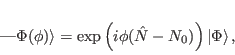
Hartree-Fock-Bogoliubov (HFB) framework, the wave function rotated in
the gauge space is defined as [2,7]
As demonstrated by Lipkin [13], the minimized energy, obtained by the full variation after the particle-number projection
(VAPNP), can also be obtained through an auxiliary Routhian,
Similarly, after the Lipkin method is executed,
the particle-number-projection (PNP) of the final Lipkin state
![]() gives an approximation to the exact VAPNP state. The
advantage here is that the time-consuming exact PNP calculation is
performed only once, that is, the Lipkin method allows for obtaining
the full VAP result by effectively performing only the PAV
calculation. Apart from the total energy, other observables must be
calculated by using the PNP of the Lipkin state.
gives an approximation to the exact VAPNP state. The
advantage here is that the time-consuming exact PNP calculation is
performed only once, that is, the Lipkin method allows for obtaining
the full VAP result by effectively performing only the PAV
calculation. Apart from the total energy, other observables must be
calculated by using the PNP of the Lipkin state.
As suggested by Lipkin [13], the simplest and manageable
ansatz for the Lipkin operator ![]() has the form of a power
expansion,
has the form of a power
expansion,
Up to now, the LN method
was frequently used to estimate values of ![]() (traditionally denoted by
(traditionally denoted by ![]() ).
However, this method relies on calculating the average values of
).
However, this method relies on calculating the average values of
![]() and
and
![]() , and, thus, at higher
orders (
, and, thus, at higher
orders (![]() ) evaluation of these terms becomes cumbersome and
impractical.
) evaluation of these terms becomes cumbersome and
impractical.
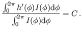
The essence of the original Lipkin method is different, namely, it relies
on deriving expressions
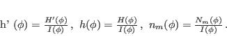
for ![]() that ``flatten'' the
that ``flatten'' the ![]() -dependence
of the reduced Routhian kernel
-dependence
of the reduced Routhian kernel ![]() , that is,
, that is,
The equivalency of the energy obtained by minimizing the auxiliary
Routhian with that resulting from the exact VAPNP can be
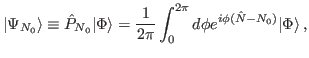
demonstrated as follows. In the HFB frame, the
PNP state can be obtained in a standard
way [2]
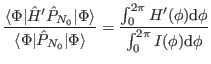
Since for the state projected on ![]() , the average value of the Lipkin
operator (8) is, by definition, equal to zero, we also have that
, the average value of the Lipkin
operator (8) is, by definition, equal to zero, we also have that
| (13) |
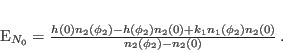
The largest contributions to integrals
in Eq. (12) come
from the vicinity of the origin due to the largest
weight [17]. Therefore, we can evaluate Lipkin parameters ![]() using the gauge-rotated intrinsic states near the origin. This also
avoids the singularities caused by vanishing overlaps [8]. As
an example, at second order one obtains the Lipkin parameter,
using the gauge-rotated intrinsic states near the origin. This also
avoids the singularities caused by vanishing overlaps [8]. As
an example, at second order one obtains the Lipkin parameter,
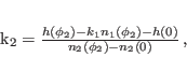
Similarly, at order ![]() , we evaluate Lipkin parameters
, we evaluate Lipkin parameters ![]() ,
,
![]() , using a set of
, using a set of ![]() small gauge angles
small gauge angles ![]() ,
,
![]() . In practice, in this work, we use equally spaced
values of
. In practice, in this work, we use equally spaced
values of
![]() , and at each order we check the eventual
dependence of results on the maximum gauge angle used,
, and at each order we check the eventual
dependence of results on the maximum gauge angle used, ![]() .
If at the given order
.
If at the given order ![]() , the convergence of the expansion of Lipkin
operator (8) is reached, the resulting parameters do not
depend on the choice of the maximum gauge angle. We test the
convergence based on this philosophy.
, the convergence of the expansion of Lipkin
operator (8) is reached, the resulting parameters do not
depend on the choice of the maximum gauge angle. We test the
convergence based on this philosophy.
The above derivations are strictly valid only in the case of energy
kernels given by average values of the Hamiltonian. However, in the
nuclear EDF approach, most often density-dependent interactions and interactions
different in the particle-hole and particle-particle channels are used, and thus
poles may occur when the overlaps between gauge rotated intrinsic
states vanish (it may happen at gauge angle
![]() ) [4,8,9,10]. In such a case,
none of the standard methods, like VAPNP, PAV, LN, or Kamlah, nor the
Lipkin method discussed here, are strictly valid, and a construction
of regularized functionals is mandatory [9,10].
) [4,8,9,10]. In such a case,
none of the standard methods, like VAPNP, PAV, LN, or Kamlah, nor the
Lipkin method discussed here, are strictly valid, and a construction
of regularized functionals is mandatory [9,10].
In this sense, the Lipkin method that employs appropriately small
maximum gauge angles, which do not approach the hypothetically
dangerous region of ![]() , can be regarded as a certain
regularization method. By doing so, we regularize the energy kernels
in terms of the analytic continuation of the Lipkin energy kernels to
the full range of gauge angles. Obviously, at large gauge angels, the
calculated and regularized energy kernels can then be different. Thus
the tests of convergence of the Lipkin operator are meaningful only
in the region of gauge angles where the energy kernels are not
ill-defined.
, can be regarded as a certain
regularization method. By doing so, we regularize the energy kernels
in terms of the analytic continuation of the Lipkin energy kernels to
the full range of gauge angles. Obviously, at large gauge angels, the
calculated and regularized energy kernels can then be different. Thus
the tests of convergence of the Lipkin operator are meaningful only
in the region of gauge angles where the energy kernels are not
ill-defined.
We note here that the minimization of the average Routhian
(7) with respect to the HFB state ![]() can be
performed by solving the standard HFB equation with additional
higher-order terms added, see Appendix A. We also note that
Lipkin parameters
can be
performed by solving the standard HFB equation with additional
higher-order terms added, see Appendix A. We also note that
Lipkin parameters ![]() must be determined in each HFB iteration
(for each current state
must be determined in each HFB iteration
(for each current state ![]() ), in such a way that at the end
of the HFB convergence they correspond to the final self-consistent
solution, and thus parametrically depend on it. However, this
dependence does not give rise to any additional terms in the HFB equation,
because the derivation of the Lipkin method is based on treating them as constants,
cf. discussion of the LN and Kamlah methods in Ref. [19].
), in such a way that at the end
of the HFB convergence they correspond to the final self-consistent
solution, and thus parametrically depend on it. However, this
dependence does not give rise to any additional terms in the HFB equation,
because the derivation of the Lipkin method is based on treating them as constants,
cf. discussion of the LN and Kamlah methods in Ref. [19].
An exactly solvable two-level pairing model offers an ideal environment to test qualitative properties of the Lipkin VAPNP method. The results presented in Appendix B show that in such a schematic model, the higher-order Lipkin VAPNP method is able to reproduce correctly the exact VAPNP ground-state energies, both in weak and strong pairing regimes, everywhere apart from the immediate vicinity of the closed shell. This gives us confidence in applications of this method in more involved cases of actual nuclei, which is discussed in the next section.
Jacek Dobaczewski 2014-12-07